Flow Field Reduced-Order Modeling: Compressing 480 Snapshots into Dominant Modes

Building the Foundation

Initially, I wanted an intuitive way to observe fluid dynamics anytime in both browsers and terminals. Traditional commercial CFD software requires complex meshing and heavy differential equation solving, making real-time web interactivity impractical. To solve this, I wrote a lightweight solver from scratch in JavaScript: FlowLab: Rebuilding a Lattice Boltzmann Method Solver. Rather than discretizing the continuous Navier–Stokes equations directly, I adopted the Lattice Boltzmann Method (LBM). The resulting solver runs smoothly at 60 FPS in the browser, allowing interactive vortex manipulation in lid-driven cavity flow.

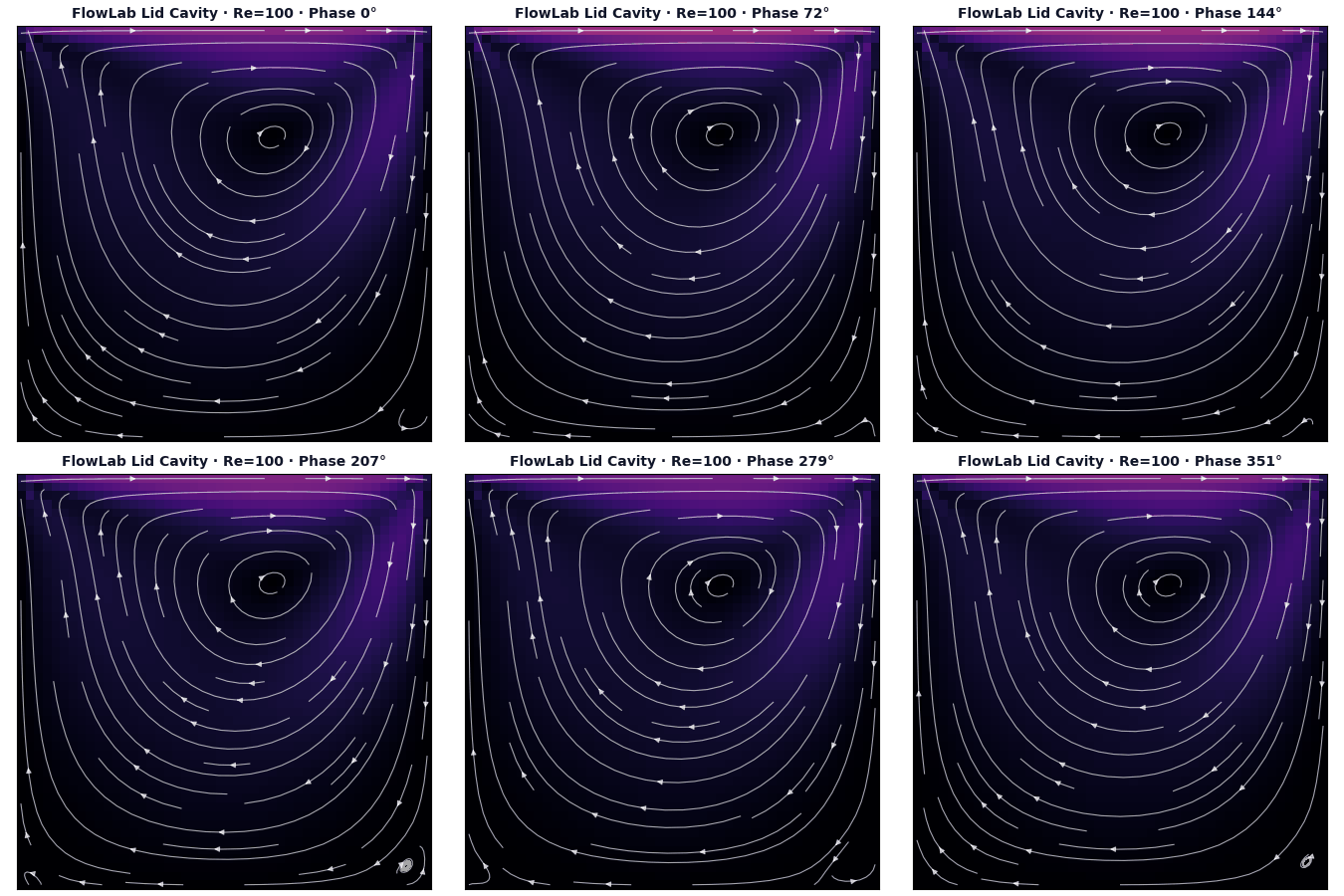
However, when investigating unsteady flows subject to periodic boundary perturbations, I ran into a practical bottleneck: massive data volume. Capturing transient vortex shedding required saving full velocity snapshots every few milliseconds. A single simulation run quickly accumulated gigabytes of raw data. Beyond heavy storage demands, post-processing hundreds of discrete snapshots sequentially was cumbersome and inefficient.

This led to a central question: given the strong coherent structures in periodic flow, can we compress hundreds of complex flow snapshots into a handful of dominant spatial ‘skeleton modes’—analogous to video compression—and extrapolate future flow evolution without re-running the underlying solver equations?

To achieve this, I built FlowROM, a dedicated flow field reduced-order modeling and forecasting toolkit.

Understanding the Lattice Boltzmann Method (LBM)

Where conventional CFD treats fluid as a continuum governed by partial differential equations, the Lattice Boltzmann Method (LBM) views fluid as microscopic particle ensembles interacting on a regular discrete lattice. I implemented the standard 2D D2Q9 lattice model: the domain is discretized into Cartesian cells where particle velocity distributions move in 9 discrete directions (one rest particle, four axial directions, and four diagonals).

At each timestep, the algorithm executes two straightforward operations:

1. Collision: Particles arriving at the same lattice node collide, relaxing their directional distributions toward a local Maxwellian equilibrium;
2. Streaming: Post-collision distributions advance along their respective velocity vectors to neighboring nodes.

Summing the 9 directional distributions recovers local macroscopic density; momentum-weighted averaging yields macroscopic velocity. Because it eliminates the need to solve a global Poisson pressure equation, LBM is inherently parallel and computationally lightweight. Using FlowLab, I ran a cavity flow with sinusoidal lid velocity perturbations, waited for periodic limit-cycle oscillation to stabilize, and recorded snapshots every 10 timesteps—yielding 480 transient velocity field snapshots as the benchmark dataset.

How FlowROM Works

FlowROM does not solve governing fluid equations directly; rather, it serves as an algorithmic toolkit designed for spatial dimensionality reduction and temporal forecasting. It consists of two core components:

1. Proper Orthogonal Decomposition (POD)

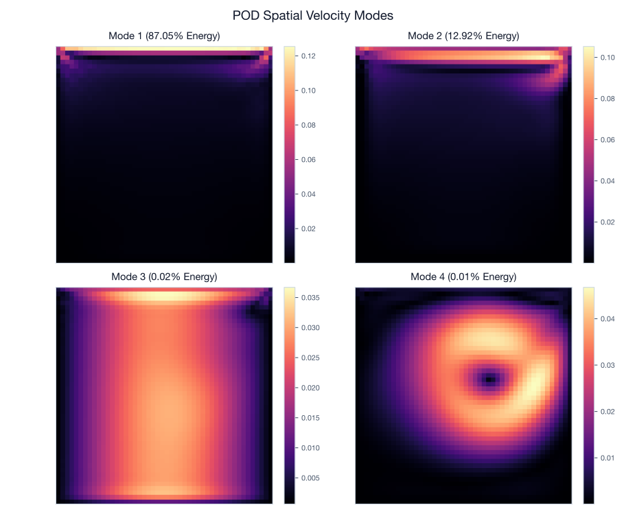
POD performs spatial dimensionality reduction. After subtracting the time-averaged mean flow from the 480 snapshot matrix, Singular Value Decomposition (SVD) extracts orthogonal spatial mode bases ranked by kinetic energy content:

• The raw velocity field contains thousands of spatial degrees of freedom per frame;
• Retaining just the top 8 POD spatial modes alongside their 8 scalar temporal coefficients compresses the representation by nearly $50\times$;
• Reconstructing the flow from these 8 modes achieves a fluctuation error of only ~0.1%.

2. Dynamic Mode Decomposition (DMD)

While POD efficiently compresses historical data, it does not inherently provide a dynamical model for forward temporal extrapolation. To predict future flow evolution, I integrated Dynamic Mode Decomposition (DMD). DMD fits a best-fit linear operator mapping snapshot $x_k$ to $x_{k+1}$:

• Frequency Identification: DMD extracts the dominant oscillation frequencies and growth/decay rates from sequential snapshots with high spectral precision;
• Autonomous Forward Extrapolation: Starting from the final snapshot of the training window, DMD advances the dynamical state forward in time without calling the CFD solver, forecasting flow field evolution across the subsequent 4 oscillation cycles.

Train-Test Split Strategy

I partitioned the dataset chronologically: the first 320 frames (~8 oscillation cycles) formed the training set, while the final 160 frames (4 full cycles) were reserved strictly as an unseen holdout test set.

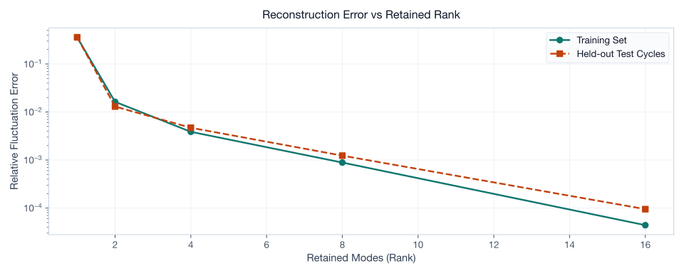
In standard machine learning workflows, a random 80/20 train-test split is common practice. However, in periodic fluid dynamics, random temporal sampling causes severe data leakage. Because periodic flow repeats cyclically, a randomly held-out frame is nearly identical to adjacent training frames. The model would merely perform temporal interpolation rather than learning true underlying physical dynamics.

By enforcing a contiguous future block of 4 full cycles as the holdout set, the model is forced to extrapolate autonomously from the boundary of known data into the unseen future, rigorously testing its predictive fidelity.

Lessons from a 1-Mode Failure

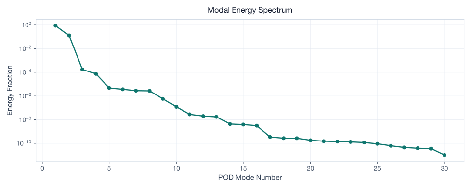
Examining the cumulative energy spectrum, Mode 1 alone accounted for 87.0% of total fluctuation kinetic energy. Initially, this suggested that a single spatial mode might suffice to capture the flow. However, evaluating the 1-mode reconstruction on the holdout test set resulted in a massive 35.97% error—losing over a third of the dynamic fluctuation details:

Retained Modes	Training Set Error	Unseen Test Set Error
1 Mode	35.98%	35.97% (Severe Distortion)
2 Modes	1.63%	1.30% (Dramatic Improvement)
4 Modes	0.39%	0.47%
8 Modes	0.09%	0.12%

Why did the 1-mode model fail so dramatically despite holding 87% of the energy? Periodic vortex dynamics represent limit-cycle orbits in phase space. Describing a circular or elliptical trajectory in 2D space requires at least a pair of orthogonal spatial bases—analogous to expressing circular motion via $\cos(\omega t)$ and $\sin(\omega t)$. A single spatial mode cannot capture phase propagation.

Incorporating Mode 2 immediately collapsed the holdout reconstruction error from 35.97% down to 1.30%. This demonstrates that model order reduction cannot rely purely on energy threshold heuristics; it requires physical pairing of conjugate modes validated on unseen holdout datasets.

Dual-Denominator Error Analysis

When evaluating the 4-cycle autonomous forward extrapolation accuracy of DMD, I tracked two distinct error metrics:

• Relative to full total velocity field: 0.10% (appearing near-flawless)
• Relative to zero-mean fluctuation field: 1.41% (accurately reflecting oscillation deviation)

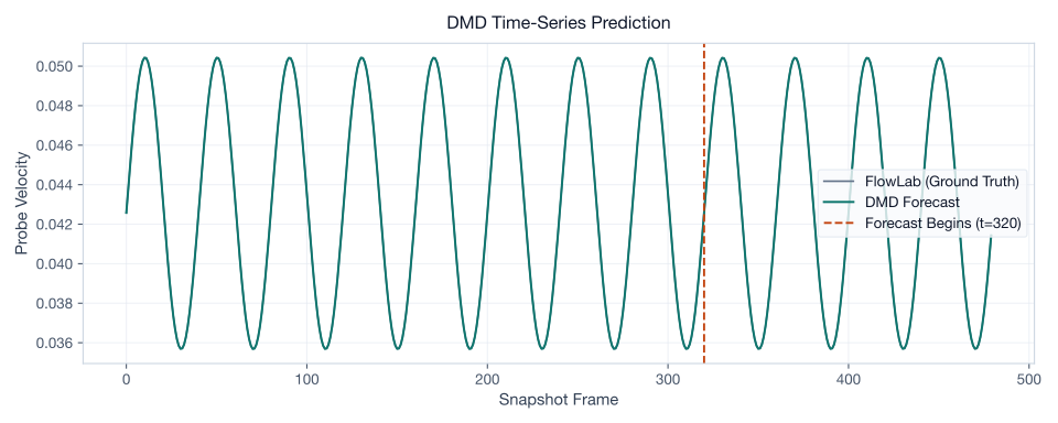
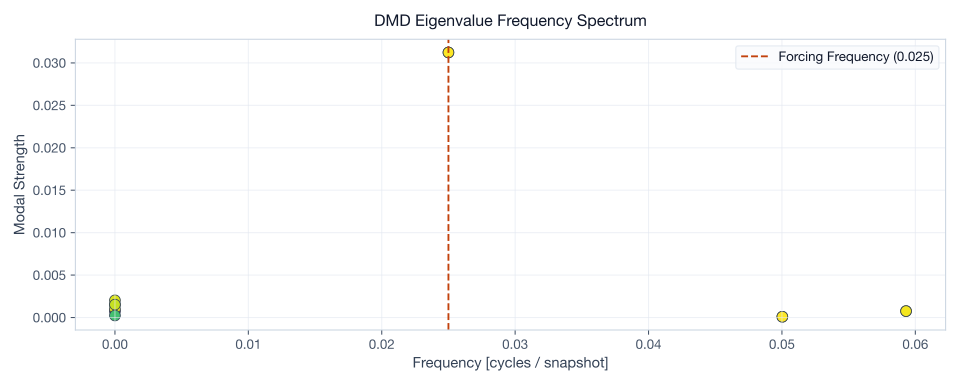
In driven cavity flow, the mean velocity field accounts for the vast majority of absolute kinetic energy. When evaluating error against the total velocity magnitude (large denominator), the resulting error is under 0.1%.

However, when evaluating the accuracy of unsteady dynamic forecasting, the static mean flow must be subtracted to assess fluctuation errors directly. Against the fluctuation denominator, the error is 1.41%. Reporting only the 0.10% metric risks masking extrapolation drift behind static background flow. Both metrics must be reported transparently.

Unit Testing & Verification

Because FlowLab served as both data generator and benchmark reference, bugs in the reduction pipeline could easily go unnoticed if tested exclusively against simulated flow data.

To prevent circular verification, I instituted synthetic unit tests with analytical solutions:

1. Synthetic Rank-2 Matrix Test for POD: Validates that orthogonal spatial modes and singular values reconstruct the analytical matrix to machine precision;
2. Synthetic Harmonic Signal Test for DMD: Validates that continuous frequencies, growth rates, and dynamic modes are recovered exactly from pure sinusoidal inputs.

Because these synthetic test cases have exact analytical ground truths, any discrepancy isolates bugs directly to the reduction algorithms rather than data quality issues.

Scope and Limitations

All data in this study originated from a $48 \times 48$ lattice cavity flow—representing a single geometry, single Reynolds number, and low-speed regime. It is not a surrogate for full-scale external racecar aerodynamics, nor can it directly predict complex 3D vehicle wakes. Extending this methodology to vehicle aerodynamic campaigns will require parameterized datasets covering varying ride heights, velocities, and yaw angles across multi-condition training sets.

Nonetheless, the established pipeline—leakage-free temporal partitioning, POD spatial basis compression, DMD frequency identification, conjugate mode pairing, and dual-denominator error verification—provides a robust and reproducible foundation for reduced-order modeling.

Code and Reproduction

The project is open source on GitHub: gaoflow/flowrom

git clone https://github.com/gaoflow/flowrom.git
cd flowrom
node scripts/generate-snapshots.mjs
python3 scripts/analyse.py

Application Context

In long-duration unsteady CFD simulations, full transient flow field data (e.g., velocity and pressure fields) can quickly exceed dozens of gigabytes, making storage expensive and real-time control design intractable.

By processing 480 flow snapshots through the FlowROM pipeline, Proper Orthogonal Decomposition (POD) extracts just 8 orthogonal spatial modes, achieving a nearly $50\times$ compression ratio while retaining over 99.9% of flow kinetic energy. Combined with Dynamic Mode Decomposition (DMD), the system extracts dominant vortex shedding frequencies with high precision and accurately forecasts future flow evolution across four full cycles without resolving the underlying Navier–Stokes / LBM equations.

As I encounter more complex aerodynamic scenarios in future coursework and research, I will continue expanding this framework.