Simulating the Kármán Vortex Street in Fluent

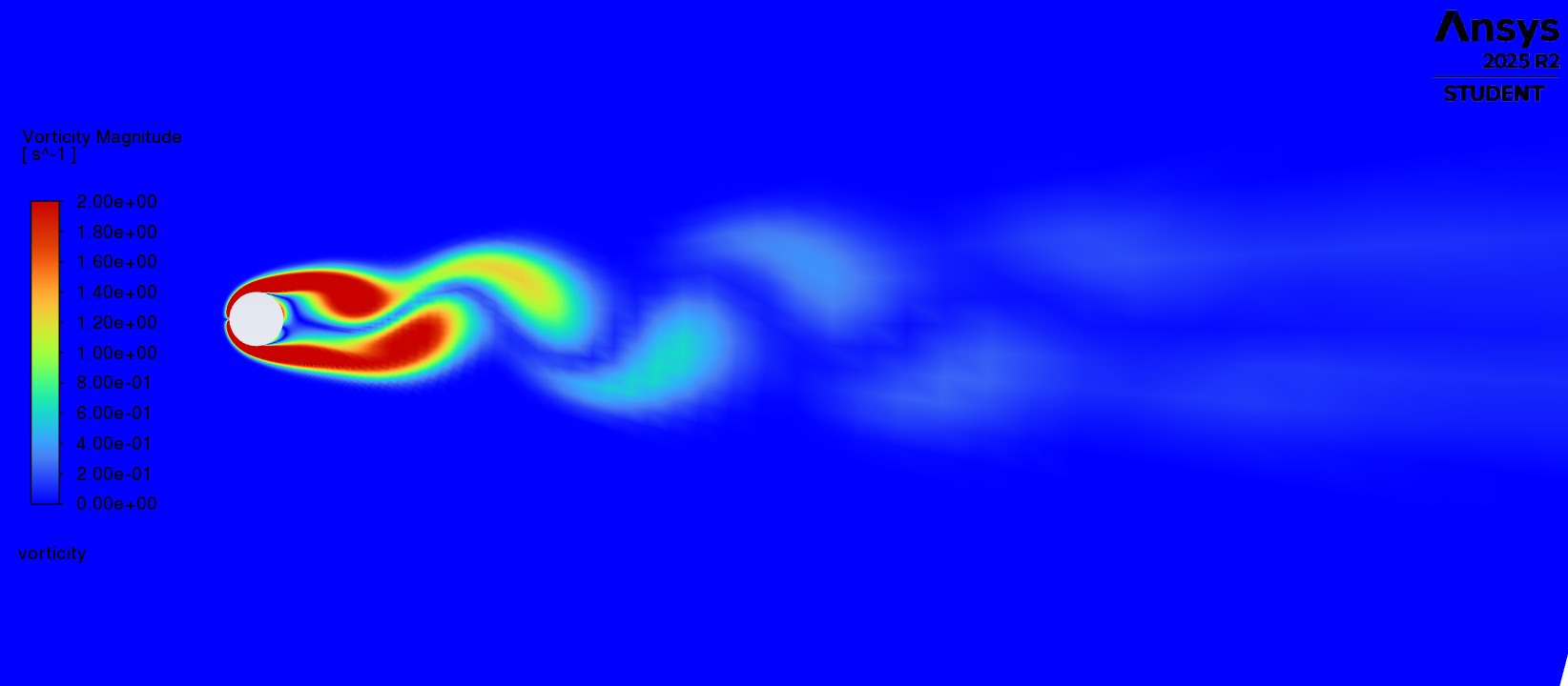
This is my lab record from the Computational Fluid Dynamics course in the Spring 2026 semester.

Assignment Description

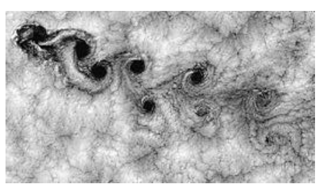
The assignment began with a concrete fluid dynamics question: when fluid flows past a cylinder, why does it sometimes leave a steady wake, yet at other times shed vortices alternately from both sides? The instructor introduced the phenomenon using natural Kármán vortex streets. Islands act as bluff bodies that force atmospheric flow separation, shedding vortices alternately from either side and leaving visible periodic structures downstream.

The assignment juxtaposed two distinct flow regimes: first, solve steady flow past a cylinder at $Re=40$, checking convergence, mass conservation, velocity, streamlines, vorticity, pressure, and drag; next, increase the Reynolds number to 150 using a transient solver to monitor lift and drag, characterizing the unsteady wake periodicity with a dimensionless parameter. That parameter is the Strouhal number evaluated later.

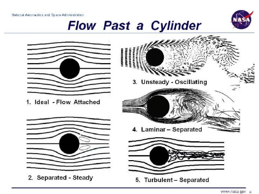
Two-Regime Framework

I structured the instructor’s requirements into two cylinder flow cases: a steady symmetric wake at $Re=40$, and an unsteady Kármán vortex street at $Re=150$. I set up two Fluent cases (steady and transient) and triggered the vortex street using a controlled perturbation. After the simulations completed, I digitized the retained monitor screenshots frame-by-frame to reconstruct the force histories. The results were mixed: the vortex shedding frequency yielded $St=0.155$, but the drag was 29.3% lower than the experimental benchmark. The frequency was sound, whereas the pressure drag lacked precision.

Following the assignment guidelines, both cases shared a common quadrilateral mesh of 20,200 nodes, with approximately 100 elements along the cylinder circumference. The fluid density was 1 kg/m³ and the cylinder diameter was 1 m. The transient case also used Fluent Adapt to refine the downstream wake region, with a residual convergence target set to $10^{-3}$.

$Re=40$ Steady Benchmark Case

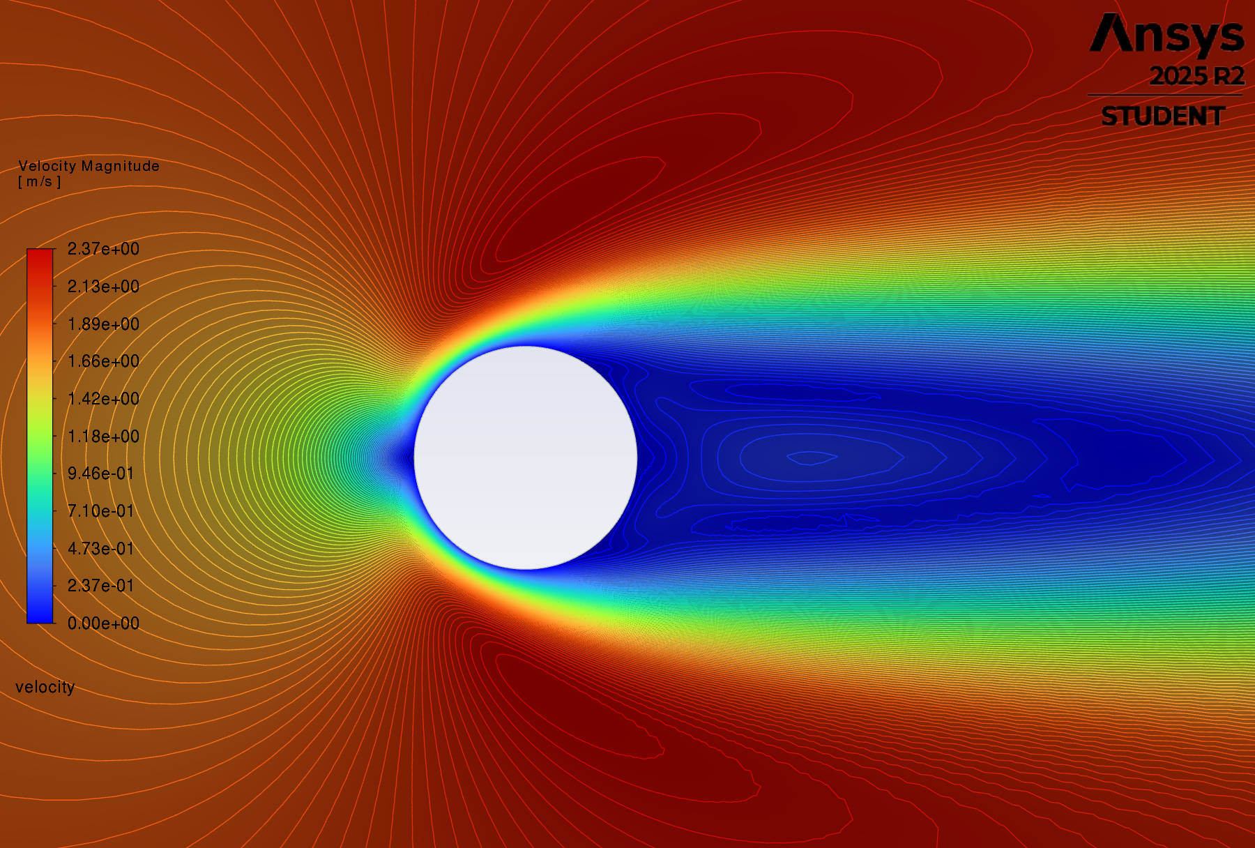
At $Re=40$, the wake remains steady and top-bottom symmetric across the centerline. Two closed recirculation zones form behind the cylinder; top and bottom pressures cancel out, resulting in zero net lift. This steady result later served another purpose: providing an independent control when analyzing the drag discrepancy at $Re=150$. The drag decomposes as follows:

Component	Force	Coefficient
Pressure	2.0100 N	3.2816
Viscous	1.0615 N	1.7330
Total	3.0714 N	5.0146

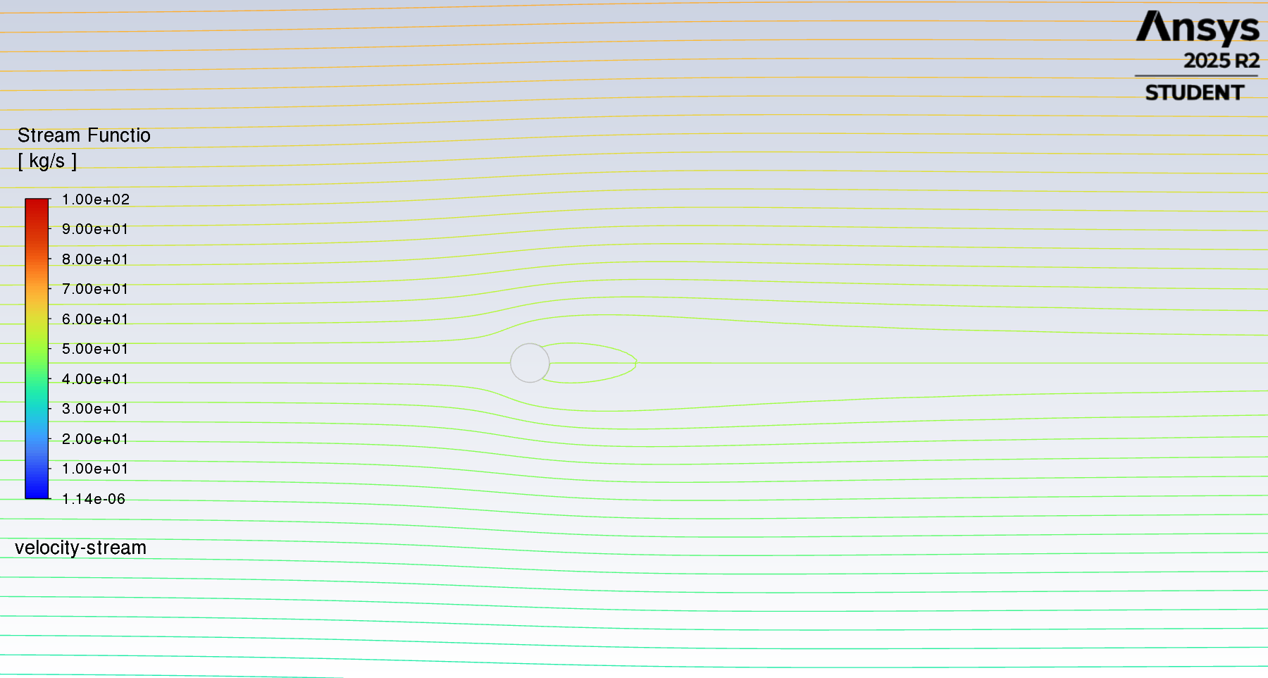
The $Re=150$ Case

Real physical flow at $Re=150$ is inherently unstable, spontaneously developing alternating shedding vortices behind the cylinder. However, in the numerical model, the mesh, inlet boundary, and cylinder geometry are all perfectly symmetric about the centerline. With neither governing equations nor boundary conditions breaking symmetry, the numerical solution can linger in a quasi-symmetric state for an extended duration. The instability that occurs naturally in physical experiments does not emerge immediately in such a simulation.

Waiting for roundoff errors to trigger instability would risk exceeding our limited computational budget. Therefore, after initialization, I manually introduced an asymmetry using a patch: adding a $+0.2$ m/s transverse ($Y$) velocity in the downstream quadrant where $X>0.5$ m and $Y>0$.

The peak velocity immediately after perturbation was

$$\sqrt{1^2+0.2^2}\approx1.02\ \text{m/s},$$

consistent with the initial contour plots.

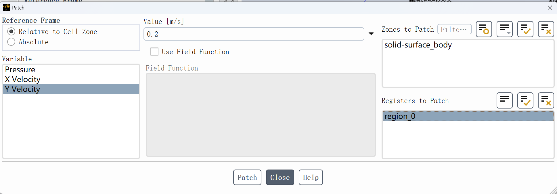
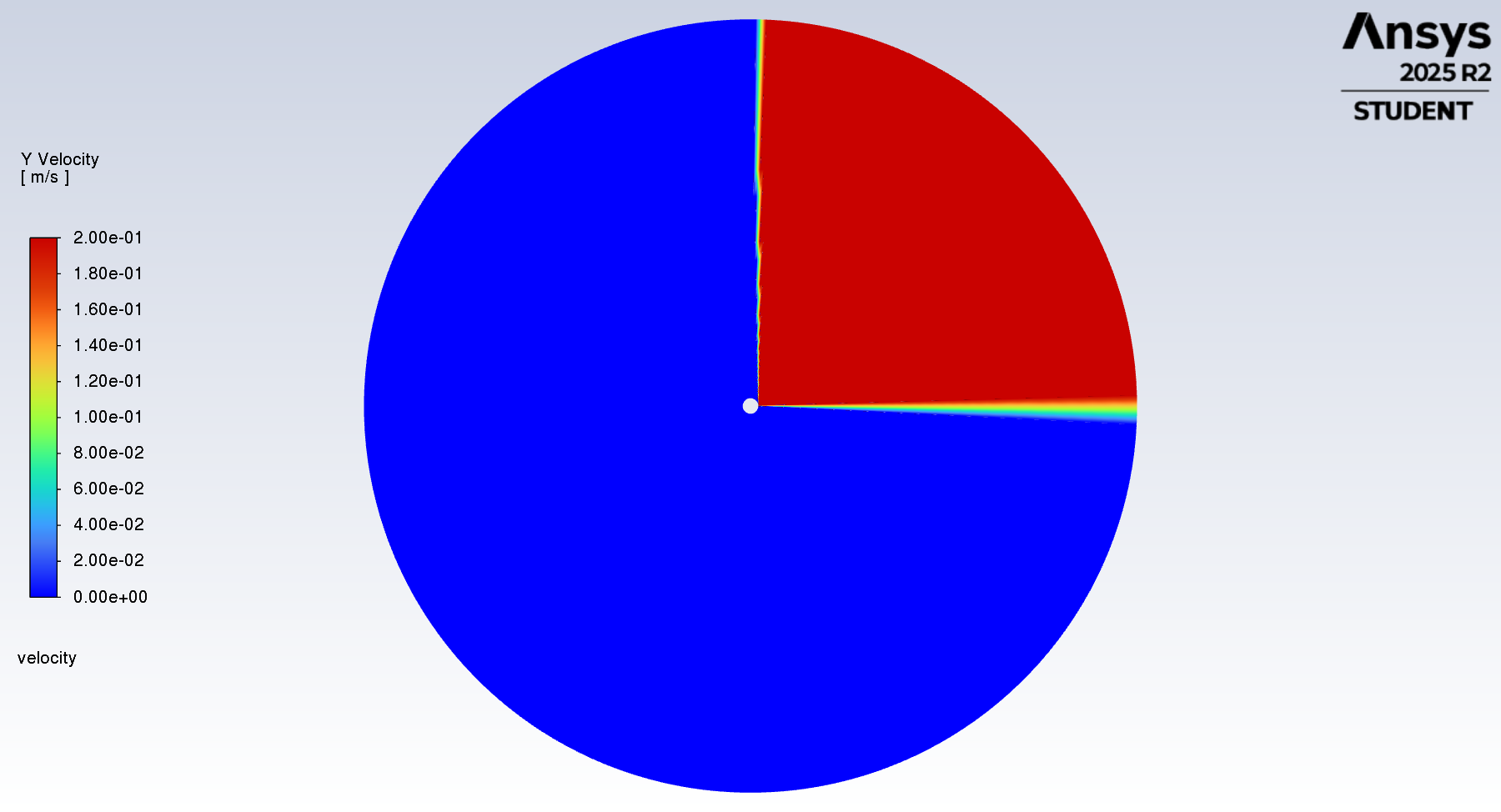
This perturbation serves solely to seed the initial phase for vortex shedding without dictating the asymptotic shedding frequency. Once vortex shedding reaches limit-cycle oscillation, lift oscillates symmetrically around zero, demonstrating that the artificial bias does not persist into the fully developed state. Had the perturbation exerted a continuous bias, the lift history would remain offset to one side.

Transition from Symmetric Wake to Vortex Street

The complete output spans 400 frames, playing for 13.33 seconds at 30 fps. Initially, the wake behind the cylinder remains nearly symmetric. As the perturbation amplifies, the upper and lower shear layers roll up alternately, shedding vortices in sequence and culminating in a stable Kármán vortex street.

Determining $St=0.155$ from the Lift History

Vortices shed alternately from the top and bottom surfaces of the cylinder; each vortex pair corresponds to one complete oscillation of the lift coefficient around zero. In the fully developed regime, the amplitude stabilizes at approximately $\pm0.117$. Using the most direct zero-crossing approach on the curve after $t>40$ s, I identified the upward zero-crossing timestamps across six full cycles. The mean period was 6.44 s, yielding

$$f=0.155\ \text{Hz},\qquad St=\frac{fD}{U}=0.155.$$

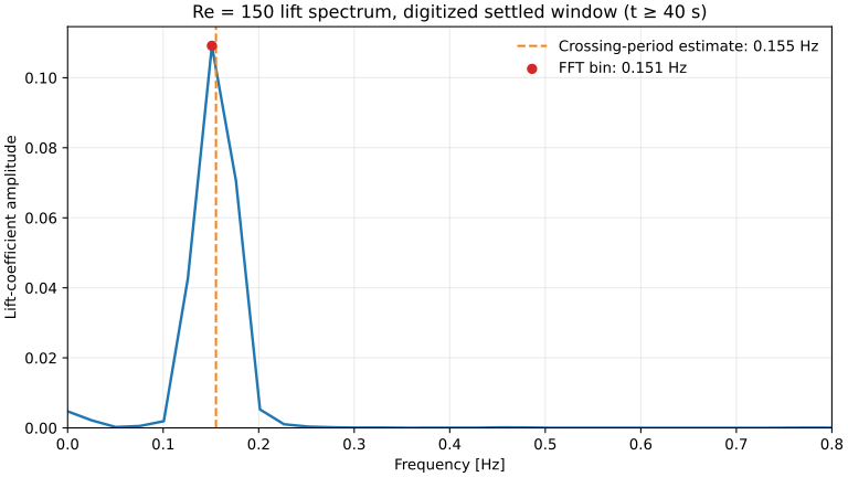
To further substantiate this shedding frequency, I performed a Hann-windowed FFT on the same digitized lift history. For 670 samples with a frequency resolution of 0.0252 Hz, the dominant non-zero spectral peak was located at 0.151 Hz, falling within the same frequency bin as the zero-crossing result. While the lift history quantifies cycle period, instantaneous field contours reveal spatial structures. The vorticity contour captures alternating shear-layer roll-up, while the pressure contour illustrates stagnation high pressure coupled with alternating downstream low-pressure vortex cores.

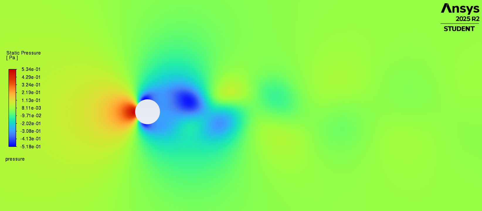
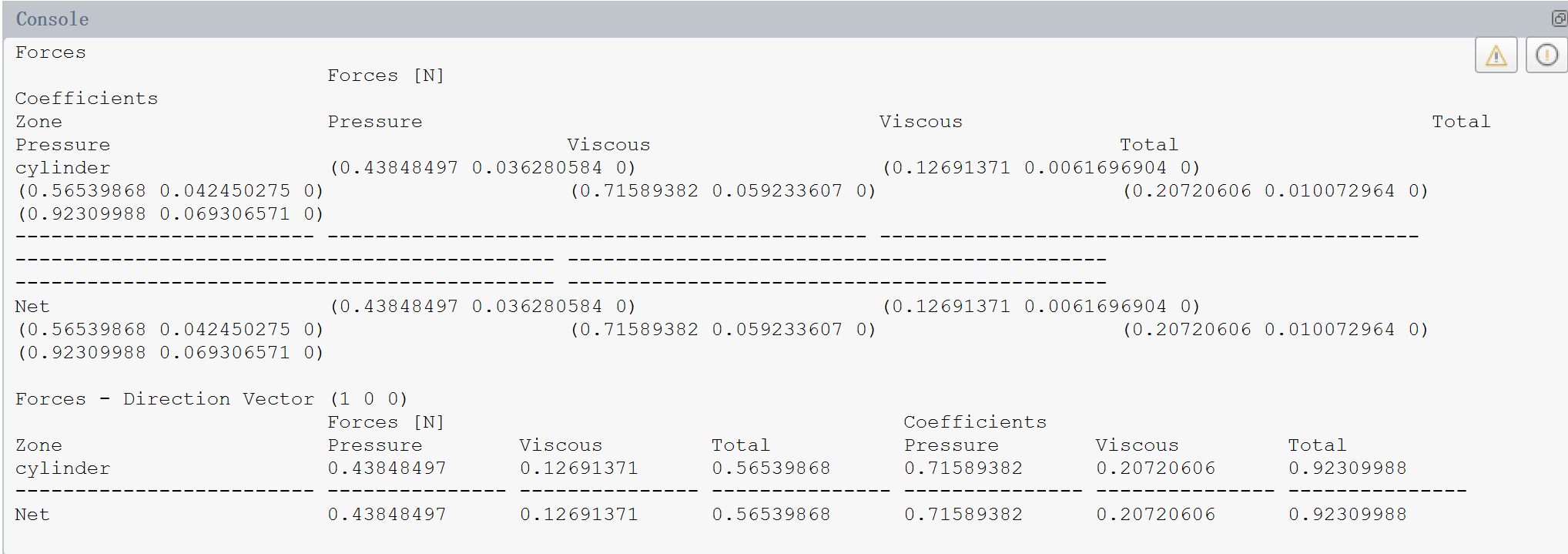
The forces at the final time step for $Re=150$ were:

Component	Force	Coefficient
Pressure	0.4385 N	0.7159
Viscous	0.1269 N	0.2072
Total	0.5654 N	0.9231

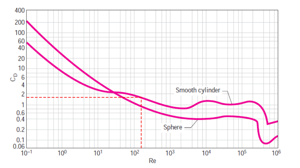
The experimental reference corresponds to roughly 0.8 N under these conditions, meaning the simulation underpredicted drag by 29.3%. This deficit stems primarily from the pressure component: pressure drag accounts for 78% of total computed drag, indicating that the crux lies in base pressure recovery behind the cylinder rather than wall viscous friction. A similar directional underprediction appeared in the $Re=40$ steady case: computed drag was 3.07 N against ~4.2 N from reference charts, an underestimation of 26.9%. That a steady and a transient case exhibited comparable deficits suggests the $Re=150$ discrepancy was not merely an artifact of sampling at a single instant in time.

I hypothesize that numerical dissipation plays a major role. A coarse mesh combined with relatively relaxed transient convergence tolerances can damp shedding vortices and artificially elevate wake base pressure, reducing the front-to-back pressure differential. Another common pitfall: residual convergence merely signifies that Fluent solved the discrete algebraic system for that time step—it does not imply that integrated forces are physically accurate. Equations can converge cleanly on a mesh that remains too coarse.

The exported forces and coefficients in both cases satisfied $C_D=F_D/0.6125$. However, the theoretical dynamic pressure references for $Re=40$ and $Re=150$ are 2.0 and 0.5, respectively. This indicates that both runs reused a single static set of reference values in Fluent without recomputing dynamic pressure per case. Consequently, comparing these raw coefficients directly against literature charts would conflate differing definitions. This analysis compares dimensional forces instead, as reference areas cancel out under identical geometry.

Furthermore, the pressure coefficient of 3.2816 happened to be close to the total drag coefficient of 3.28 in the reference chart, but the two represent entirely different physical quantities. Numerical proximity cannot substitute for validation unless both share an identical definition. Therefore, this article evaluates exported pressure force, viscous force, and total drag against the course reference curve under consistent geometry, rather than taking raw $C_D$ values at face value.

Final Numerical Results

Metric / Verification Item	Result
Re=40 steady convergence	53 iterations, residuals $< 10^{-6}$
Re=40 mass imbalance	$5.84\times10^{-9}$ kg/s
Final $C_L$ (digitized vs. exported)	0.075 vs. 0.069
Final drag (digitized vs. exported)	0.555 N vs. 0.565 N
Shedding period	Six cycles, standard deviation 0.03 s
Strouhal number	0.155

Summary

Through this hands-on course assignment, I first solidified my familiarity with the fundamental ANSYS and Fluent workflow. Starting from geometry, meshing, and boundary condition specification, I configured steady and transient solvers, monitored residuals, lift, and drag, and inspected the resulting velocity, pressure, and vorticity fields. Second, I developed a deeper understanding of CFD methodology: residual convergence merely indicates that the discrete algebraic equations were solved, not that integrated engineering quantities are fully accurate. Shedding frequency and drag must also be evaluated separately: this simulation captured a reasonable vortex shedding frequency, yet pressure drag retained a substantial discrepancy relative to empirical reference data. I recognized the simplifications and limitations inherent in this case: a 2D laminar formulation utilizing a single grid and a fixed 0.2 s time step without grid or time-step refinement studies. The calculated $St=0.155$ was derived from only six shedding cycles, and the existing mesh lacked sufficient resolution to finely capture the boundary layer governing separation points. Thus, while these results effectively elucidate vortex shedding mechanisms and validate frequency, the drag values should not be treated as high-precision data.

This remains a quintessential canonical CFD benchmark. In subsequent work, I plan to reproduce this case using OpenFOAM—replicating both the $Re=40$ steady wake and $Re=150$ Kármán vortex street while adding systematic mesh, time-step, and domain independence refinements, extending sampling durations, and exporting lift/drag histories directly. This will turn this simplified coursework baseline into a foundation for rigorously isolating the effects of grid resolution, time stepping, and numerical schemes on shedding frequency and drag.