Building an FSAE Cooling System from Scratch

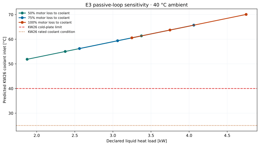
Origins: How to Lower Water Temperature to 25 °C on a 40 °C Track Day?

The origin of this investigation began when I joined the Vinci EcoDrive team to take charge of powertrain cooling. I immediately ran into a tough practical dilemma: the motor and inverter supplier specified a strict ceiling requiring coolant inlet temperature not to exceed 25 °C.

Yet in a midsummer track environment at 40 °C, if we rely solely on passive ram-air flow through sidepod radiators, how could coolant ever drop below ambient temperature in steady state?

This was an architectural conflict that was physically impossible before a single line of calculation was written. To provide the team with a clear engineering judgment grounded in a mathematical model, I modeled everything from the E3 passive loop to the E7 dual-temperature architecture and E8 catalog selection, using quantitative data to explain why blind procurement had to be halted.

E3: Sufficient Flow, but Thermally Impossible

The E3 setup combined two Boyd 6310G3 heat exchangers, two SPAL brushless fans, and one Pierburg CWA150 water pump.

I integrated four core physical elements into a single coupled model:

• Intersection of fan performance curves with core and duct hydraulic resistance curves;
• Intersection of pump head curves with parallel radiator and motor branch resistance curves;
• Interpolation within manufacturer thermal conductance data;
• A 1D finite-volume loop accounting simultaneously for advection, heat sources, heat rejection, and thermal storage.

The air-side operating point settled at 6.56 m³/min and 45.6 Pa per radiator; total coolant flow was 10.03 L/min, with the most restrictive motor branch still receiving 4.16 L/min. Judging solely by air and coolant flow rates, this combination appeared compliant.

The real issue lay in the temperature boundary conditions. E3 assumed 40 °C ambient air entering the radiators, whereas the AMK KW26 inverter demanded a coolant inlet temperature of 25 °C. Without active refrigeration, a radiator can only asymptotically approach ambient temperature; it is physically impossible for a passive radiator to cool fluid below ambient in steady state.

In other words, before the solver executed a single iteration, this passive architecture already contained a fundamental physical contradiction.

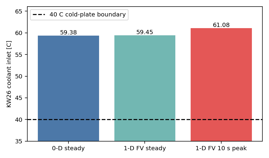
The numerical model quantified the exact severity of the failure:

• Under the minimum thermal load condition, the KW26 inlet temperature still reached 51.86 °C;
• The 80-cell baseline loop stabilized at 59.45 °C, with a peak coolant temperature of 63.87 °C;
• Under a 10 s, 6.0 kW peak surge condition, maximum coolant temperature escalated to 68.18 °C;
• Under adverse fan curves, the fan operating curve failed to intersect the system resistance curve entirely.

Consequently, I formally rejected E3. What was rejected was the passive architecture itself, not the individual pumps, fans, or radiators, which could still serve in other configurations.

Proving E3 Was Not a Numerical False Negative

Before issuing a rejection, I needed to prove conclusively that this failure was a physical impossibility rather than a modeling mistake.

Under baseline conditions, the 80-cell loop received 3,061.53 W of heat, rejected 3,061.43 W through the radiators, with the remaining 0.105 W altering system thermal storage. The algebraic energy conservation residual was only $3.2\times10^{-12}$ W.

During the peak surge condition, 6,000 W was injected, radiators rejected 3,595.51 W, and the remaining 2,404.49 W was absorbed into thermal capacitance. The resulting temperature rise stemmed strictly from the governing energy equations without any artificially imposed thermal ramps.

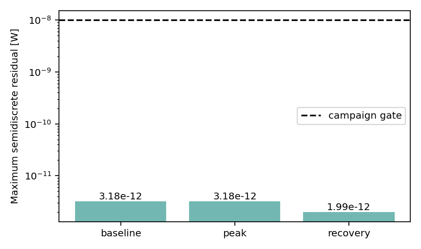
I also independently refined spatial discretization and time stepping:

Check	Variation between finest two levels	Requirement
20→40→80→160 cells	0.029 K	$<0.1$ K
Three time steps	0.018 K	$<0.1$ K
80-cell model vs independent steady-state equation	0.078 K	$<0.1$ K

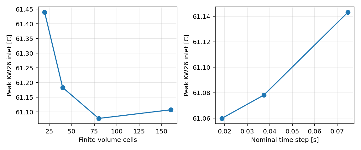
These results demonstrate that the failure was not an artifact of the chosen discretization scale. However, they only prove that the model solved its own equations stably; they cannot convert unknown thermal loads into measured inputs.

E7: Splitting the System into Two Temperature Levels

After E3 failed, I stopped expecting a single passive loop to serve both the KW26 and DD5, and split the architecture instead:

• An active low-temperature loop for the KW26, with an inlet boundary of 25 °C;
• A passive high-temperature loop for the two DD5 motors, allowing inlets between 40–60 °C;
• A refrigerant loop transferring heat and compressor power from the KW26 to the high-temperature side;
• Independent air paths for the condenser and DD5 radiators.

Rather than locking in a specific chiller unit, E7 swept across assumed parameter ranges:

Parameter	Sweep range
KW26 liquid thermal load	0.500–2.000 kW
Ambient heat leak	0–0.300 kW
Refrigeration COP	1.5–3.0
Required evaporator capacity	0.500–2.300 kW
Compressor power	0.167–1.533 kW
High-temperature side total heat rejection	2.041–6.582 kW
DD5 inlet temperature	48.7–57.4 °C
DD5 derating	8.7%–17.4%

All combinations achieved balance within the declared equations. Therefore, E7 proves only one thing: the dual-temperature architecture is numerically feasible across these assumed ranges. It lacks specific data on evaporators, condensers, control valves, accumulators, parasitic power, and packaging constraints, so it cannot be directly converted into a hardware solution.

E8: Mapping Assumptions to Public Catalog Components

E8 built a steady-state reference for the three loops using public catalog data. Primary components included the Masterflux SIERRA03-0982Y3 compressor, Danfoss B3-012 plate heat exchanger, Bosch PCE high-temperature pump, Pierburg CWA150 pump, Boyd 6310G3 core, and SPAL fans.

To emphasize: these component models served solely as model inputs and do not imply that the team had finalized procurement.

E8 evaluated two KW26 evaporator thermal loads: 0.820 kW and 2.300 kW. On the DD5 side, the liquid thermal load from the two motors was swept from 1.374 kW to 2.749 kW. The nominal model achieved compliance across all declared flow rates, temperatures, heat exchanger UA values, compressor capacities, pump heads, and fan settings.

However, passing a single nominal operating point is insufficient. I then used a bisection search to locate the exact transition point where each parameter shifted from “pass” to “fail”:

Boundary	Last passing point	First failing point
Condenser fan minimum command	68.0168%	68.0161%
DD5 fan minimum command	43.5217%	43.5208%
Shared available UA across three B3 units	67.0258%	67.0251%
KW26 loop maximum pressure loss	1.26000 bar	1.26001 bar
Maximum liquid heat load for two DD5 motors	3.13434 kW	Above 3.13434 kW

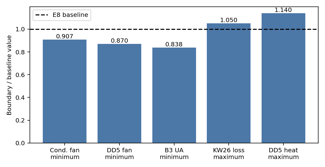
These decimal values represent numerical boundaries within deterministic equations, not requirements for hardware control precision. Real-world vehicles must handle sensor errors, manufacturing tolerances, fouling, control latency, and environmental fluctuations, requiring far larger engineering margins.

Why Univariate Margins Cannot Be Directly Combined

Combining the five “last passing points” simultaneously would enter a parameter combination the model never validated. To analyze parameter coupling, I computed five $5\times5$ interaction grids:

• Condenser fan command vs available B3 UA;
• DD5 fan command vs DD5 liquid heat load;
• KW26 thermal load vs low-temperature loop pump head;
• Ambient temperature vs KW26 thermal load;
• DD5 air allocation vs available radiator conductance.

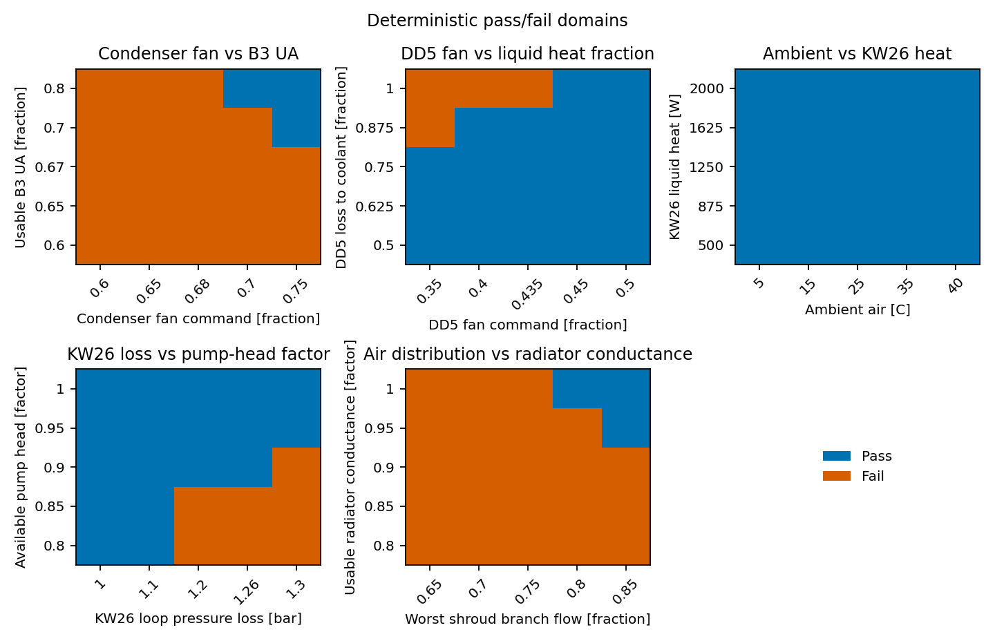
The conclusion is straightforward: when one parameter degrades, the minimum requirement on another parameter increases. The five univariate boundaries represent five different cross-sections and cannot be treated as five independent allowances usable at the same time.

I also applied twelve larger perturbations to confirm that failures occurred in the expected directions. For instance, the condenser fan passed at 70% but failed at 65%; available B3 UA passed at 70% but failed at 65%; and the KW26 loop pressure loss failed when increased from 1.20 bar to 1.30 bar.

Surrogate Duct: OpenFOAM Qualified the Method Only

Once the system architecture achieved numerical convergence, CFD became appropriate to answer how air moves through the fan, shroud, and radiator core.

I built an isolated 3D surrogate duct: the fan was modeled with a full-face pressure jump, the core with an isotropic Darcy–Forchheimer porous medium, and four mesh levels maintained identical geometry and boundary conditions.

Mesh	Cell count	Core flow rate (m³/s)	Core pressure drop (Pa)
Coarse	7,440	0.143580	32.654
Medium	53,940	0.134869	34.961
Fine	431,520	0.130726	36.073
Extra Fine	3,481,920	0.129484	36.078

Between the fine and extra-fine meshes, flow rate varied by 0.959% and pressure drop by 0.0145%. Global mass imbalance on the extra-fine mesh was $1.39\times10^{-5}$%, with a final time-window drift of $3.24\times10^{-5}$%.

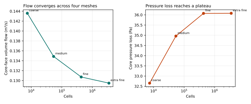
This result demonstrates only that on this idealized surrogate duct, the fan and porous core methodology passed mesh and conservation checks. The model lacks real sidepod geometry, measured freestream velocity, core non-uniformity, hot air recirculation, and conjugate heat transfer, so it cannot represent E8 on-car duct performance.

Why Procurement Remains Unjustified

What E8 validated is a steady-state model built from public data and explicit assumptions. To approve procurement, the following missing data must be supplied:

Missing data	Recommended path to supply
Actual KW26 heat rejected to coolant	Calorimeter test bench or manufacturer map
DD5 water jacket heat fraction	Independent calorimetry for left and right motors
Installed pump and core curves	First-party complete curves or physical tests
Dynamic driving cycles	Synchronized logging of speed, torque, flow rate, temperature, and ambient
Installed aerodynamic path	Frozen CAD, measured boundaries, and screened architecture
Control and failure modes	Derating tests for fans, pumps, compressors, and valves

Public materials lack KW26 loss maps at target operating points, DD5 heat split fractions to the water jacket, and pump/heat exchanger curves across complete operating envelopes. Without these data, numerical compliance cannot be translated into hardware adequacy.

How This Study Reshaped My Workflow

The most critical outcome of E3 was identifying the physical contradiction between 40 °C air and a 25 °C coolant inlet before embarking on complex calculations. E7 demonstrated that a dual-temperature architecture could achieve mathematical balance within assumed ranges. E8 then showed that even with public catalog hardware, the steady-state reference may offer only narrow localized margins.

Consequently, I now prioritize validating thermal loads and real operating conditions first, followed by architecture screening, physical component and control validation, and finally installed CFD for sidepods and ducts.

More expensive and complex models cannot compensate for undefined inputs. Disqualifying flawed architectures early with low-cost models, then focusing computational resources on viable solutions, remains the core methodology derived from this work.