Investigating Ground Effect with Image Vortices
I built a ground-effect Vortex Lattice Method (VLM) tool.
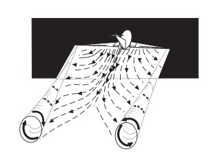
Ground Effect in Formula 1
When watching F1, we often hear about the concept of “ground effect.” The closer a wing is to the ground, the stronger the downforce tends to be. The question I was curious about is: why does a flat road surface alter the aerodynamic forces on the wing above it? And why do the results cease to be reliable when getting too close to the ground?
On a real race car, the underfloor, wheels, diffuser, and edge seal leakage simultaneously influence the airflow. Putting the entire car directly into a model makes it hard to see what the ground itself is doing. Therefore, based on the method of image vortices, I wrote a low-order Vortex Lattice Method (VLM) tool to first study a simple rectangular wing.
From 2022 to 2025, F1 cars used shaped Venturi floor tunnels to enhance ground effect:
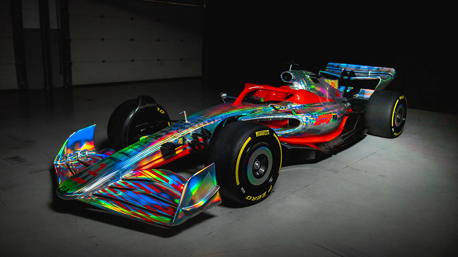
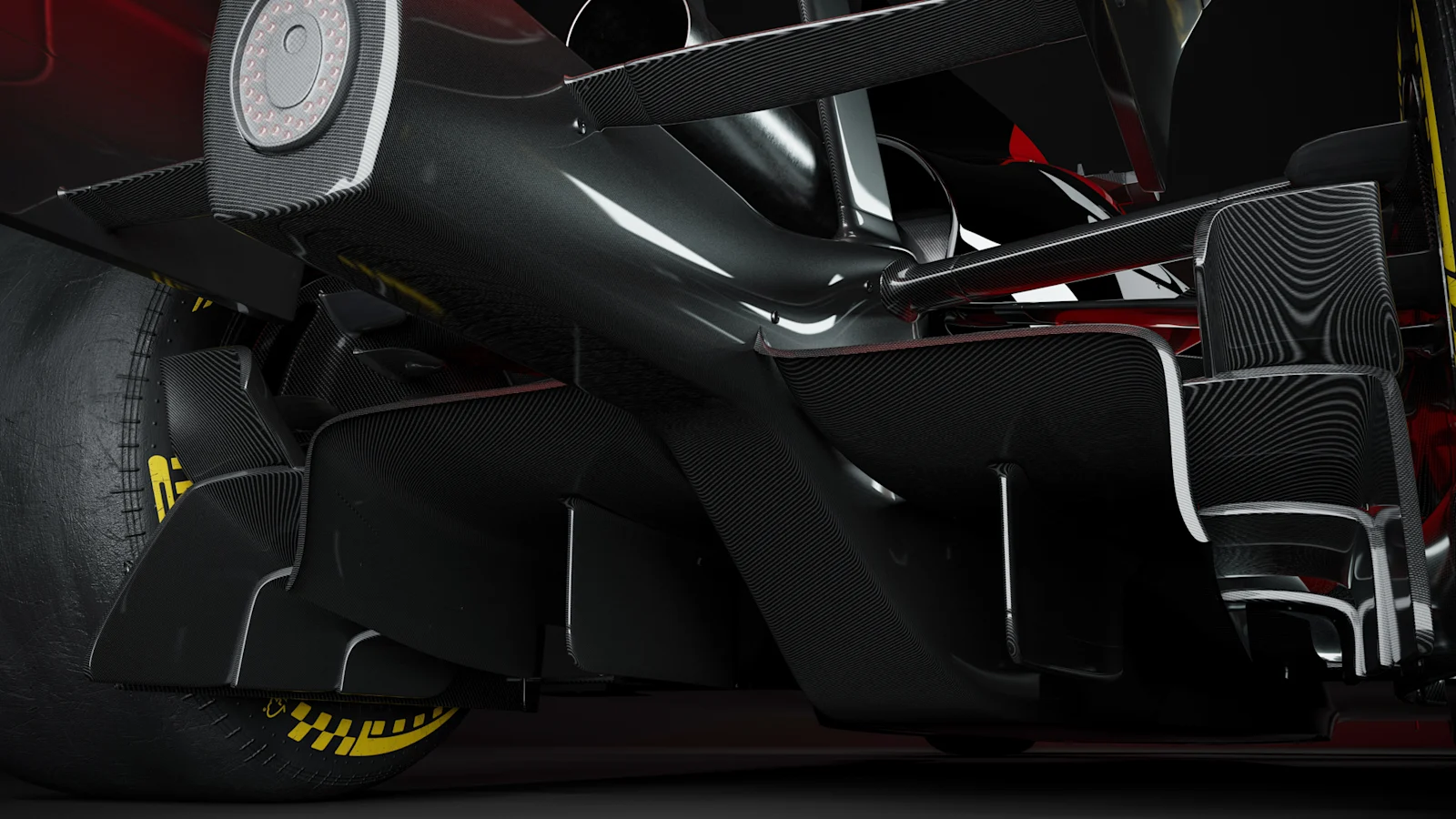
The 2026 technical regulations switch to flatter floors and larger diffusers. Ground effect does not disappear; it is simply weaker than under the previous regulations. The image below focuses on the rear of the car, also provided solely for background context.
Simplifying the Problem to a Rectangular Wing
Assume the simplest model: a thin rectangular wing facing the oncoming flow at a fixed angle of attack. Initially placed far from the ground, it gradually descends while keeping all other conditions constant. I wanted to observe three things: 1. how the spanwise load changes, 2. how much total lift increases, and 3. what induced drag penalty is paid to produce the same amount of lift.
I didn’t import CAD models or replicate a specific generation of F1 floor; those are overly complex, so I chose the simplest geometry for initial exploration. In the code, my wing has zero thickness, sweep, or twist. The chord is set to , span , and angle of attack fixed at . This simplification allows isolating ride height without introducing interference from tires, diffusers, or the chassis. Inverting the wing turns the force into F1 downforce; since my primary interest is in how ground proximity alters loading, whether the force points up or down does not affect the ground-effect mechanisms discussed here.
Due to the simplicity of the model, it is intended only for observing trends. Lacking viscosity and flow separation, it cannot predict at what ride height a real race car will stall.
What Is a Vortex and How Is It Generated?
Simply put, a vortex is a mass of rotating air spinning around an axis. Air can translate backward while swirling. Smoke, clouds, and vapor can visualize the rotation, but the smoke itself is not the vortex; it merely tracks the air’s motion.
When a wing generates lift, the upper surface has lower pressure and the lower surface has higher pressure. Near the wingtips, the high-pressure air underneath curls around the tips toward the low-pressure region above. After leaving the wing, the air continues to roll up, eventually forming two trailing wake vortices rotating in opposite directions. NASA’s explanation of downwash and the FAA’s wake turbulence description describe this process.
To make the formation process more intuitive, I asked AI for help, and it generated a very clear animation that I found quite effective, so I included it here. The animation illustrates how the pressure difference drives the wingtip crossflow and how that crossflow rolls up into trailing vortices.
How VLM Represents a Wing
Real wakes do not naturally form neat, straight lines. To reduce computational cost, VLM approximates the lift and downwash produced by a segment of the wing using horseshoe vortices. The transverse segment of a horseshoe vortex is called the bound vortex, while the two trailing lines represent wake vortices. I discretized the rectangular wing into 64 uniform spanwise segments, placing a horseshoe vortex on each segment. The bound vortex is placed at the quarter-chord line, the collocation point checking flow tangency is placed at the three-quarter-chord line, and the trailing vortices extend 80 chord lengths downstream.
During the solve, each vortex induces velocity at all other positions. Combining these mutual influences yields a system of linear equations:
Matrix records the aerodynamic influence coefficients between vortices, and is the vector of unknown circulations across the 64 segments. Vector on the right represents the boundary conditions (sharing the letter with the span defined earlier). After solving for the circulation distribution, I calculate lift using the Kutta–Joukowski theorem, and estimate induced drag by summing circulation and wake-induced downwash across the span.
How Image Vortices Represent the Ground
The ground imposes only one fundamental boundary condition on the flow: air cannot penetrate the surface. In terms of velocity, the vertical velocity at the ground must be zero.
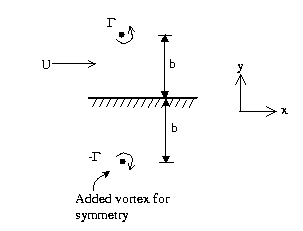
My approach places a set of image vortices beneath the ground plane. Each image vortex is positioned symmetrically below its corresponding real vortex above the ground, with opposite circulation. The vertical velocity induced by a real vortex at the ground plane is exactly cancelled by its image vortex. This satisfies the impermeability condition without needing to mesh the ground.
The figure below illustrates the same principle with a 2D vortex. The above the ground is the real vortex, and below is the image vortex, both at distance from the wall.
I first placed the wing at to obtain a baseline virtually free of ground influence. Then, I gradually lowered the ride height down to , computing 14 states in total. Here, denotes the distance from the quarter-chord line to the ground.
Observing Spanwise Load Distribution
After solving for circulation, I first compared load distribution shapes. Each curve below is normalized by its own maximum circulation, so it shows the spanwise distribution shape rather than total lift magnitude.
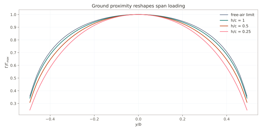
As ride height decreases, the curve becomes fuller near the wingtips. Ground proximity does not merely scale up total load; it also alters how load is distributed along the span.
Examining the Three Metrics Separately
The left plot shows the lift increase at fixed angle of attack relative to free flight, while the right plot shows how the induced drag penalty per unit lift changes. Both horizontal axes are , where smaller values indicate closer proximity to the ground.
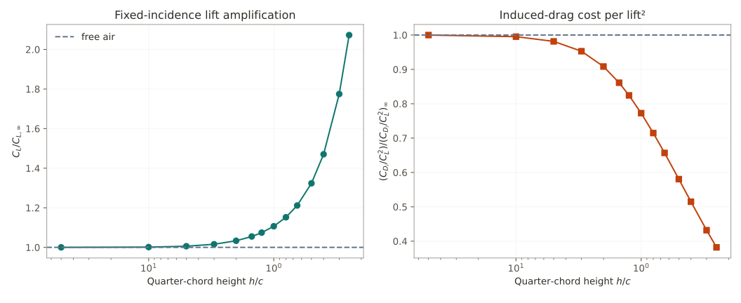
The free-stream baseline is and . When the wing drops to , increases by 32.4% to 0.3461. Absolute induced drag only increases by 1.7% to 0.00559. Concurrently, drops by 41.9%.
In short, the large reduction in the third metric is primarily driven by the larger denominator , rather than a decrease in absolute drag. Thus, I can conclude that producing the same amount of lift costs less induced drag. However, the claim that “absolute drag decreases as soon as a wing approaches the ground” does not hold here.
Verification and Discrepancy Checks
After identifying the trends, I verified whether the image vortices truly enforced the ground boundary condition, checked whether the solution recovered free-stream values far from the ground, and inspected theoretical magnitudes, panel refinement, and spanwise symmetry. I then compared the deviations:
| Check | Result | Criterion |
|---|---|---|
| Ground normal velocity residual | 0.0 | |
| vs. free-stream lift difference | 0.00335% | % |
| Difference vs. Prandtl lift-curve slope | 11.01% | % |
| Lift change from 64 to 96 panels | 0.258% | % |
| Spanwise load asymmetry error |
The solver also directly checks vertical velocity across 27 ground test points (a grid of 3 streamwise and 9 spanwise coordinates). The zero residual confirms the mirror boundary functions as expected. The 0.00335% difference between and free stream confirms that ground effects decay at large distances.
The left plot below compares the free-stream lift-curve slope against Prandtl’s lifting-line estimate, while the right plot checks grid convergence at under panel refinement.
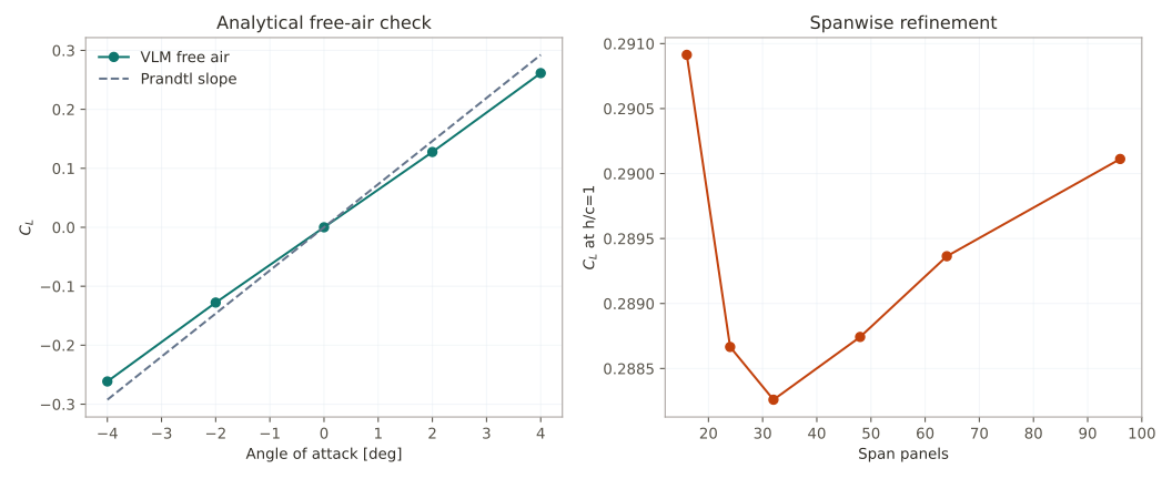
There remains an 11.01% discrepancy in the lift-curve slope. I chose not to mask it with arbitrary calibration. Increasing panels from 64 to 96 only changes lift by 0.258%, indicating that further panel refinement cannot eliminate this gap. I believe this primarily stems from the simplifications inherent in the low-order model.
Caveats on Minimum Ride Height
At , the model predicts (2.07 times the free-stream value), and the conventional span efficiency metric reaches 2.59.
In a linear model, image vortices have no flow separation constraint. As ride height continues to decrease, the numbers will only grow larger, but the model introduces no new real-world physics. The conventional free-stream efficiency expression exceeds unity here because ground presence fundamentally alters the boundary conditions. This value should only be used to compare trends, not interpreted as standard aircraft Oswald efficiency.
Therefore, I set as the lower limit of the sweep. It represents an intentional stopping point for extrapolation, not an experimentally determined breakdown height. This model can neither account for physical boundary-layer separation and stall, nor determine at which ride height they will occur.
Summary
This model is built on steady, incompressible, inviscid, and zero-thickness assumptions. It neglects road boundary layers, chassis blockage, pressure recovery, and flow separation. I treat it purely as a low-cost tool for checking directions, orders of magnitude, and numerical workflows. Real-world race car aerodynamics are vastly more complex, requiring consideration of finite thickness, chordwise loading, moving-ground boundary layers, ride height and pitch dynamics, tires, leakage, diffusers, mesh sensitivity, and flow separation.
Code & Reproducibility
This project is open-sourced on GitHub: gaoflow/ground-effect-vlm
git clone https://github.com/gaoflow/ground-effect-vlm.git
cd ground-effect-vlm
python3 -m unittest discover -s tests -v
python3 scripts/analyse.py