Estimating Cooling Loop Flow Rate Without Physical Hardware

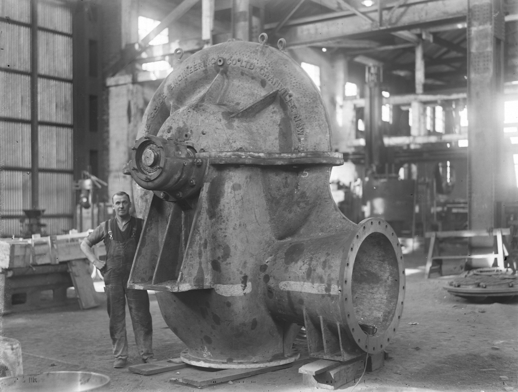
The Datasheet’s 40 L/min Is Not the Operating Reality

This project was carried out in the third month of my first year of master’s studies in mechanical engineering. Our team was discussing the cooling system for our FSAE race car. A water pump datasheet stated “maximum flow rate: 40 L/min,” and I needed to verify what flow rate would actually be achieved in practice.

That rating comes with a major caveat: near-zero discharge resistance (free delivery). Once installed in a real vehicle, coolant must pass through hoses, elbows, radiators, and narrow engine cooling jackets. It behaves much like a garden hose: short and straight, it fills a bucket quickly; lengthen it, bend it around corners, or constrict a section, and the flow drops significantly even though the water source remains unchanged.

If the flow rate is overestimated at this stage, subsequent thermal calculations—no matter how many decimal places are kept—will be evaluating the wrong operating condition. Therefore, I needed to solve this core question:

Given a pump curve and a series circuit, at what flow rate does the pump pressure head exactly match the total pressure losses across the loop?

Cooling Circuit Topology

To calculate flow rate, I decomposed the circuit into four series components: suction hose, radiator core, engine water jacket, and return hose. Connected end-to-end, coolant flows sequentially through each section before returning to the pump.

A series circuit has a key property: the flow rate is identical through every component. I only needed to calculate the pressure drop across each of the four sections and sum them up to determine the total pressure head required by the system at any given flow rate.

Component	Length	Inner Diameter	$K$
Suction hose	0.40 m	16 mm	1.5
Radiator core	0.15 m	16 mm	8.0
Engine water jacket	0.50 m	14 mm	4.0
Return hose	0.60 m	16 mm	2.0

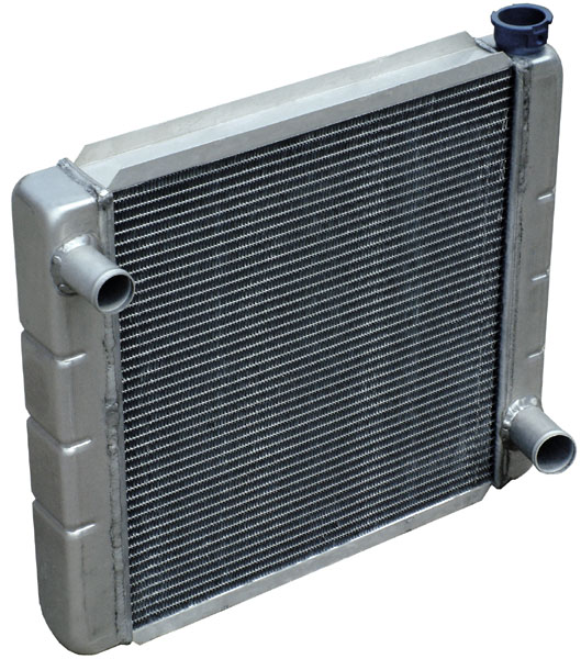
The radiator introduces substantial resistance because coolant does not simply pass through a large open cavity; instead, it is distributed into dozens of narrow micro-channels.

Converting Each Component into Pressure Drop

I calculated the pressure drop for each component using the standard Darcy–Weisbach formulation:

$$\Delta p=\left(f\frac{L}{D}+K\right)\frac{\rho V^2}{2}.$$

This equation decomposes into two parts: $fL/D$ accounts for major friction loss along the pipe walls, while $K$ accounts for minor losses from elbows, inlets, contractions, and internal passage geometry. The final dynamic pressure term $\rho V^2/2$ depends on flow velocity—as speed increases, pressure drop rises quadratically. Length, diameter, density, and velocity can all be substituted directly. The main challenge lies in evaluating the Darcy friction factor $f$, so before solving the entire loop, I verified $f$ independently.

Calculating the Friction Factor

In laminar flow, $f$ is calculated directly:

$$f=\frac{64}{Re}.$$

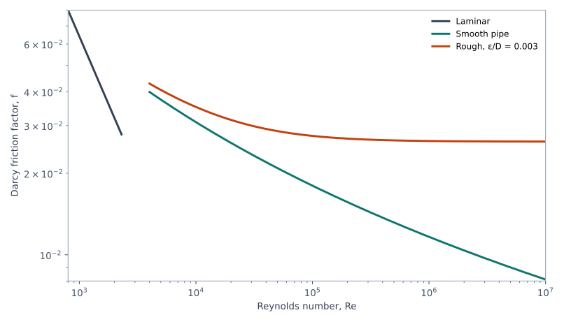
The Reynolds number acts as a gauge for flow regime: at lower values, viscosity dominates; as it increases, the flow transitions into turbulence, and pipe wall roughness begins to dictate friction. I sampled 200 points between $Re=100$ and $2300$, and the solver output matched $64/Re$ with a difference of exactly 0.0.

Turbulent flow is more complex. In the Colebrook equation, $f$ appears implicitly on both sides, requiring iterative numerical solution. I first used the Haaland approximation to provide a close initial guess, then refined it using Newton–Raphson iteration. If convergence is not reached within 50 iterations, the solver raises an error rather than returning an unverified value. After computation, I substituted each $f$ back into the Colebrook equation. Across 150 combinations of Reynolds number and relative roughness up to $Re=10^8$, the maximum residual was $3.55\times10^{-15}$. Mathematically, the solved $f$ is fully verified.

Validity Range and Domain Checks

I implemented the explicit Swamee–Jain equation as a secondary validation baseline. It claims an accuracy of $\pm3\%$, but only within the following domain:

$$5\times10^3\le Re\le10^8,\qquad 10^{-6}\le\varepsilon/D\le10^{-2}.$$

During my initial cross-comparison, I set the test domain too broadly. At very low roughness with $Re$ near $4\times10^3$, the discrepancy between the two formulations exceeded 3%. I initially suspected an error in the Colebrook solver, but soon realized these test points lay outside Swamee–Jain’s stated validity envelope. Restricting the 3% acceptance check to the equation’s declared domain brought the maximum discrepancy down to 2.83%. This discrepancy did not require modifying the Colebrook solver, but rather correcting the validation domain. It served as a reminder that empirical reference formulas have strict boundaries and cannot serve as arbiters outside their intended scope.

Having passed both verification checks, the friction factor calculation was integrated back into the four-segment pipe network.

Determining the Operating Flow Rate

I began with a trial flow rate, evaluated the pressure drop across the four segments in sequence, and summed them up:

$$\Delta p_{sys}(Q)=\sum_i \Delta p_i(Q).$$

Repeating this calculation across a range of flow rates generates the system resistance curve. As flow rate increases, system head loss rises, causing this curve to slope upward. The pump supplies head according to its own characteristic curve. The pump referenced earlier is engine-driven via a pulley, where the impeller imparts kinetic and pressure energy to the coolant. However, a pump cannot deliver a fixed flow rate irrespective of circuit resistance. This project models the pump using a representative parabolic characteristic:

$$\Delta p_{pump}=90\ \text{kPa}-cQ^2.$$

It provides 90 kPa at zero flow (shutoff head), decaying to zero pressure at 40 L/min (free delivery). The actual flow rate delivered in the system corresponds to the intersection of the pump curve and system curve:

$$\Delta p_{pump}(Q)-\Delta p_{sys}(Q)=0.$$

The solver first uses Newton–Raphson iteration to locate the root. If an iteration step jumps outside the bounding interval, it falls back to bisection for guaranteed convergence.

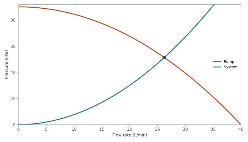
The two curves intersect at 26.22 L/min and 51.34 kPa. In other words, under these representative parameters, the 40 L/min free flow rate drops by approximately one-third once connected to the circuit.

While numerical solvers can return many decimal places, high precision does not guarantee physical correctness. I performed a fine sweep across 4,096 uniformly spaced points between 0 and 40 L/min, bracketing the sign change between the two curves. This brute-force scan bounded the intersection between 26.2173 and 26.2271 L/min, cleanly containing the Newton–Raphson result. At this operating point, pump head and system loss differ by at most $2.18\times10^{-11}\text{ Pa}$. I also verified several fundamental physical invariants: system pressure drop must increase monotonically with flow rate; adding an extra 10 kPa of static head must decrease operating flow rate; and total loop pressure drop must equal the sum of the four segment losses. With the operating point validated, the analysis turned to the practical question: which component causes the greatest restriction?

Breakdown of the 51.34 kPa Pressure Loss

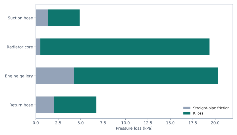
At the operating point, the suction hose loses 4.89 kPa, the radiator core loses 19.37 kPa, the engine water jacket loses 20.33 kPa, and the return hose loses 6.75 kPa. Summing these four gives exactly 51.34 kPa. The radiator core and engine jacket together account for 39.70 kPa, or roughly 77% of total system pressure drop. Looking across the entire circuit, minor loss terms ($K$) account for 43.19 kPa (84.1%), while major pipe friction accounts for 8.14 kPa (15.9%).

Therefore, under these design assumptions, reducing the restriction in the core and water jacket is far more effective than trimming a few centimeters off the hoses. However, this conclusion strictly applies to the current geometry and $K$-factor assumptions; actual proportions may shift with empirical rig measurements.

Summary

In summary, 40 L/min is merely the pump’s free delivery flow rate under zero external resistance. Once connected to a real circuit, the operating point settles at 26.22 L/min and 51.34 kPa—a reduction of about one-third. Furthermore, exploring where the pressure head is consumed revealed that roughly 77% of the 51.34 kPa is lost in the radiator core and engine water jacket; any effort to improve flow rate must target these components first.

Whenever evaluating a nominal flow rating, one must ask what pressure head that rating corresponds to, and how much pressure the actual circuit requires. Flow rate is only meaningful when the pump curve and system resistance are evaluated together. The initial discrepancy during the Swamee–Jain comparison also serves as a reminder: when results diverge, both the numerical solver and the reference equation’s domain of validity must be checked simultaneously.

Of course, 26.22 L/min is not necessarily the final vehicle design flow rate. Several simplifications remain: the pump curve is an idealized parabola, and the $K$-factors are textbook estimates rather than test-bench measurements. The model assumes steady, incompressible, single-phase flow without cavitation, aeration, or NPSH checks, and is limited to a single series loop. Next steps would incorporate empirical pump and component loss curves, followed by parallel branches and thermal network modeling for comprehensive sizing.

Code & Reproducibility

Complete source code and tests are available on GitHub: gaoflow/pipe-flow-sizing

git clone https://github.com/gaoflow/pipe-flow-sizing.git
cd pipe-flow-sizing
python3 -m unittest discover -s tests -v
python3 scripts/analyse.py

References: Formulation sources include Haaland friction approximation, Swamee–Jain cross-check, and the original Colebrook paper.