Building My First Potential Flow Model with Complex Potential

First Hearing About Flow Past a Cylinder

During a fluid mechanics lecture, our professor presented a classic example: flow past a circular cylinder. By superimposing uniform flow and an elementary flow called a “doublet,” a few equations on the blackboard pieced together the entire flow field around a cylinder. Adding a point vortex on top could even yield aerodynamic lift.

I found it fascinating at the time. How could a few invisible singularities construct an entire flow field? And how does the sign in front of the vortex dictate the resulting direction of lift? After class, combining course materials with online references, I re-derived the theory and implemented a compact “potential flow sandbox” to verify each component, focusing strictly on 2D, inviscid, incompressible flow. This also served as foundational grounding for subsequent panel methods and vortex lattice methods, which rely on the same machinery of sources, doublets, point vortices, and the Kutta–Joukowski theorem. If velocity directions or circulation signs are not properly verified at this foundational level, debugging them inside larger models becomes vastly more difficult.

Consider water flowing around a circular bridge pier. Far upstream, the water moves uniformly from left to right. As it nears the front of the pier, it decelerates and bifurcates into upper and lower streams. If both branches are completely symmetric, points with zero velocity—stagnation points—appear at the leading and trailing edges of the pier. If clockwise rotation is introduced across the flow, the velocities on the upper and lower surfaces diverge: one side accelerates with lower pressure, while the other decelerates with higher pressure, producing a net upward force.

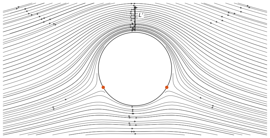
I computed this exact mechanism programmatically: uniform flow plus a doublet forms the flow past a cylinder; adding a clockwise point vortex breaks the top-bottom streamline symmetry, shifting both stagnation points (orange dots) toward the lower half of the cylinder, generating net upward lift $L'$:

Composing Four Elementary Flows into a Cylinder

Because the governing equation of potential flow is linear, elementary solutions can be directly superimposed. I first implemented four elementary flows: uniform flow carries the bulk fluid in a uniform direction; a source radiates fluid outward from a point; a doublet can be understood as a source-sink pair brought infinitesimally close; and a point vortex induces circular rotation around a point. Their respective streamlines are shown below:

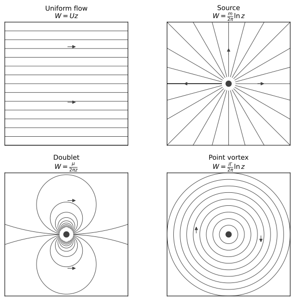
Expressed in terms of the complex potential $W(z)$, with $z = x + iy$, the velocity field is given by

$$\frac{dW}{dz}=u-iv.$$

The four elementary complex potentials are:

$$\begin{aligned} W_{\text{uniform}} &= Uz, & W_{\text{source}} &= \frac{m}{2\pi}\ln z,\\ W_{\text{doublet}} &= \frac{\mu}{2\pi z}, & W_{\text{vortex}} &= \frac{i\Gamma}{2\pi}\ln z. \end{aligned}$$

Superimposing uniform flow and a doublet “pushes open” the streamlines that would otherwise pass through the origin. The circle of radius $R$ becomes an impenetrable dividing streamline. Adding a point vortex yields flow past a cylinder with circulation:

$$W(z)=U\left(z+\frac{R^2}{z}\right)+\frac{i\Gamma}{2\pi}\ln z.$$

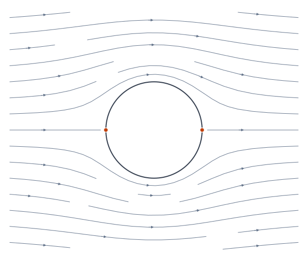
The figure below illustrates the case without circulation: fluid approaches from the left and flows around the cylinder, with orange dots marking the front and rear stagnation points. This visualizes the basic flow morphology.

Verifying Elementary Flows and Cylinder Boundary Conditions

I first selected analytical checkpoints to verify the four elementary flows. Uniform flow velocity must be constant everywhere. The velocity of a source must be purely radial, decaying as $1/r$. The velocity of a point vortex must be purely tangential, also decaying as $1/r$. The velocity of a doublet was directly compared against the analytical derivative of its complex potential. This locked down the fundamental equations and coordinate conventions. Next, I combined uniform flow and the doublet into a cylinder. The normal velocity on the cylinder surface must approach zero, and the stream function must remain constant along the boundary; far away at $1000R$, the velocity should return to the freestream value. Matching both the body surface and far-field conditions confirmed that the two elementary flows faithfully formed a solid cylinder.

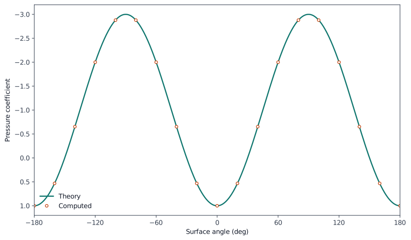
With these two verification layers passed, I computed the pressure coefficient from the surface velocity. Without circulation, the analytical solution is $C_p = 1 - 4\sin^2\theta$. At sampling points on the cylinder surface, the maximum discrepancy between the numerical implementation and the analytical curve was $2.66\times 10^{-15}$. This difference is negligible, matching the analytical solution down to the machine precision of floating-point representation.

Checking Circulation, Stagnation Points, and Lift Direction

Once the point vortex is introduced, sign conventions require active verification. Even if the sign of the vortex is flipped, the streamlines remain smooth, but the direction of rotation and the resulting lift vector will invert simultaneously. I adopted standard aerodynamic conventions: positive $\Gamma$ denotes clockwise circulation, corresponding to upward lift given by

$$L'=\rho U\Gamma.$$

Because my numerical integration contours proceed counterclockwise, converting contour integrals back to the “clockwise-positive” convention requires an explicit sign inversion. To ensure complete consistency, I verified three criteria simultaneously: the vortex-induced velocity on the right side of the cylinder must point downward; the closed line integral must recover positive $\Gamma$; and surface pressure integration must produce an upward lift force. The lift verification case used $U=1$, $R=1$, $\rho=1.225$, and $\Gamma=2\pi$—the exact parameters behind the hero figure. Based on $\sin\theta = -\Gamma/(4\pi UR)$, the stagnation points shift from $0^\circ$ and $180^\circ$ (zero circulation) to $-30^\circ$ and $-150^\circ$. The program located the two stagnation points at $-150.0^\circ$ and $-30.0^\circ$, deviating from analytical values by at most $8.9\times 10^{-16}$ rad.

I also performed contour integration along a closed circular path at $r=2.5R$. The net circulation contributions from uniform flow and the doublet along a full circle must vanish, leaving only the vortex contribution. The recovered circulation was 6.3—matching the input value $2\pi \approx 6.3$ rounded to one decimal place, with an actual residual of only $8.9\times 10^{-16}$. Finally, integrating surface pressure yielded a sectional lift of 7.7 per unit span, in exact agreement with the theoretical value of $\rho U\Gamma$, directed upward.

Verifying the Order of Accuracy for RK4

A smooth streamline plot only shows visual continuity; it does not prove the correctness of the Runge–Kutta 4th-order (RK4) integrator. Even with implementation flaws, a single trajectory integrated at a step size of 0.01 can easily appear plausible. A more rigorous method is to systematically halve the step size and observe the error convergence rate.

Launching a streamline from $(-3, 1.2)$, the trajectory was tracked using fixed-step RK4 advancing along the unit velocity direction. The streamline should theoretically remain on an invariant analytical stream function value. Halving the step size successively from 0.08 down to 0.005, I recomputed the entire streamline at each step and recorded the maximum stream function drift. For a true fourth-order method, each step-size halving should reduce the error by approximately a factor of $1/16$.

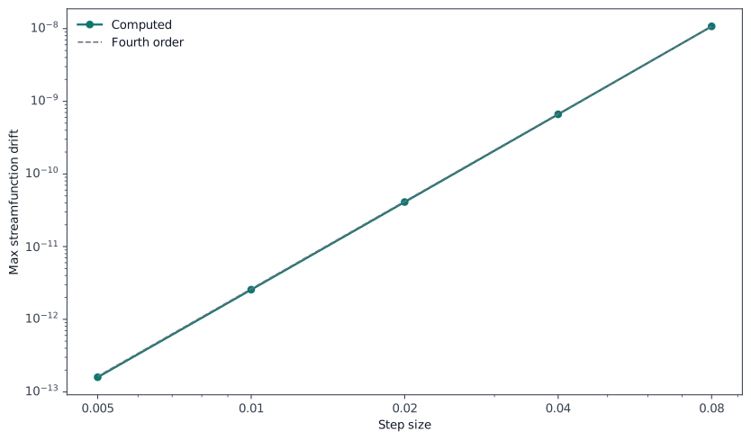
At the baseline step size of 0.01 used for verification, the maximum drift was $2.56\times 10^{-12}$; reducing to 0.005 shrank the drift by a factor of $1/16.0$, yielding an observed convergence order of 4.003. The five markers in the figure represent actual numerical computations, while the dashed line indicates the theoretical fourth-order reference slope.

The figure below shows the zero-circulation case, where the solid line is analytical theory and the points represent sampled values evaluated from the numerical velocity field.

Differences Between Ideal Streamlines and Real Wakes

Integrating surface pressure yields exactly zero drag. However, this is not a prediction of real flow around a bridge pier or physical cylinder: potential flow assumes an inviscid fluid, and this zero-drag result is d’Alembert’s paradox. The model omits boundary layers, flow separation, and wake dynamics—the primary sources of drag on a bluff body.

This clarifies a common point of confusion: potential flow past a cylinder and the Kármán vortex street share the same geometry but represent entirely different physics. The case simulated here is an idealized version—inviscid, symmetric fore-to-aft, with zero drag. Real viscous flow separates behind the cylinder and sheds an alternating vortex street, requiring Navier–Stokes CFD solvers (which I explored in a separate project).

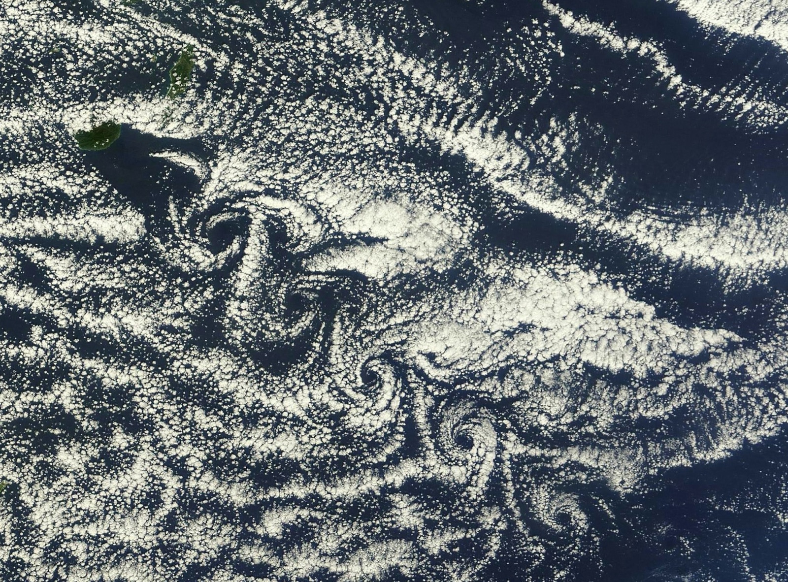
Such vortex streets occur not only in wind tunnels but also on planetary scales in the atmosphere. In November 2012, NASA’s Terra satellite captured wind blowing past Yakushima Island in Japan, with the downstream cloud deck curling into an extended trail of alternating vortices. The island acted as a giant “cylinder,” whereas the idealized potential flow model remains fore-aft symmetric without a physical wake.

Subsequent Applications

When I later developed the Hess–Smith airfoil panel method and the vortex lattice method with ground effect, I relied heavily on the same foundations: superimposition of sources, doublets, and vortices alongside Kutta–Joukowski lift. Whenever I needed to verify lift directions, I returned to this article and re-checked the analytical cylinder case—re-verifying derivatives, clockwise/counterclockwise conventions, stagnation points, and RK4 accuracy. Confirming these fundamental elements first made debugging complex surface normals, boundary matrices, and 3D meshes much more straightforward.

Code

The source code is available at gaoflow/potential-flow-sandbox.

python3 -m unittest discover -s tests -v
python3 scripts/analyse.py
python3 scripts/publish_site.py

Further Reading

• ERAU: Potential Flows covers basic potential flows, superposition, and cylinder flow, ideal for connecting equations with flow patterns.
• Oregon State: Potential Flows provides an open-textbook treatment of velocity potential, stream functions, and elementary solutions.
• Wikipedia: Potential flow around a circular cylinder summarizes velocity, pressure, and d’Alembert’s paradox for cylinder flow, useful for verifying the analytical formulas used here.