Digital Twin in Action: Reconstructing a Tensile Test in Abaqus
Coursework record: from physical tensile testing to Abaqus analysis
This is a record of a tensile testing lab completed during the Spring 2026 Materials and Behavior course.
Starting with Physical Tensile Testing
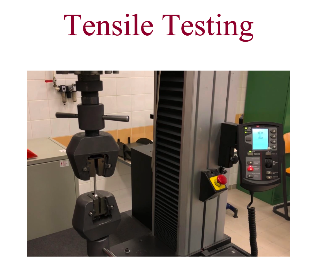
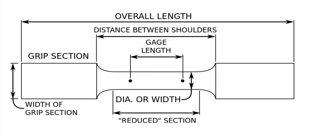
We first conducted a uniaxial tensile test on an XC48 steel dogbone specimen. The testing machine provided load and crosshead displacement, after which we measured the post-fracture dimensions and computed the engineering and true stress–strain curves using Excel. Only after obtaining this experimental curve did we begin building the Abaqus model. The question we wanted to answer was direct: can the numerical curve match the measured strain hardening, necking, and post-peak softening behavior?
Initial Curve Iteration
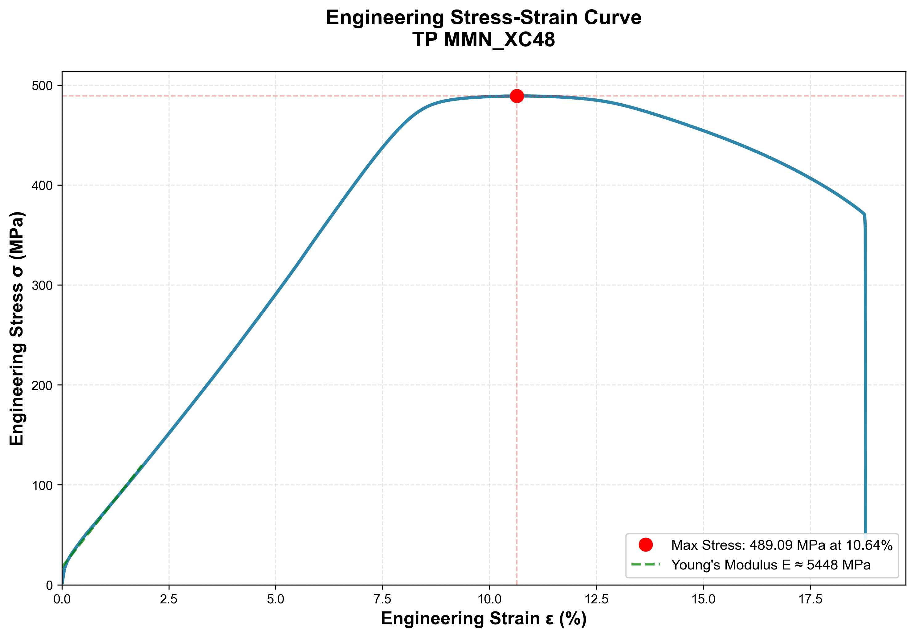
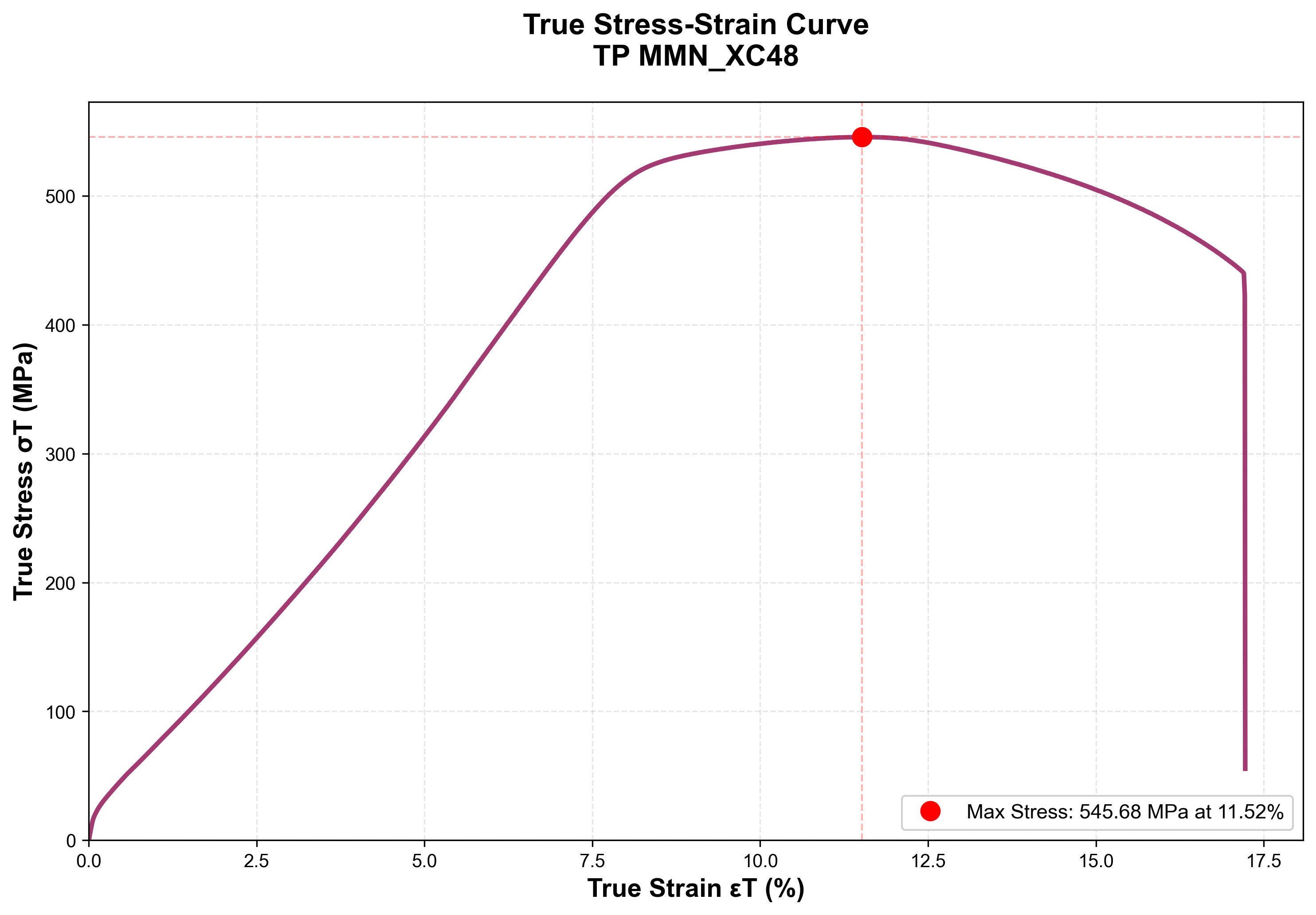
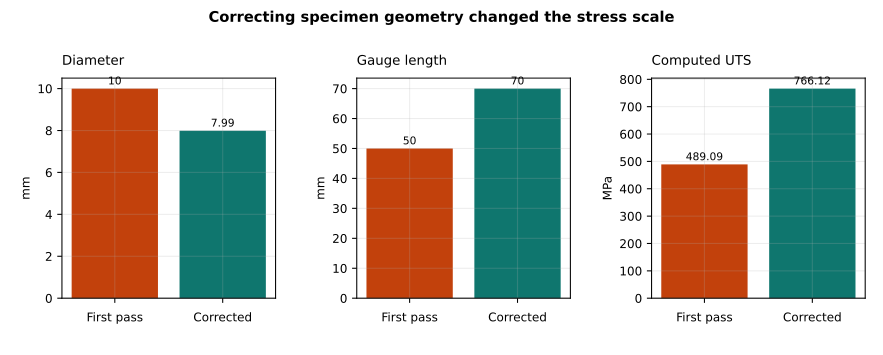
Our first calculation iteration used the same set of 1,129 raw data points but applied placeholder dimensions of Ø10 mm and a 50 mm gauge length. While the resulting curve appeared complete, the peak engineering stress reached only 489.09 MPa, with a peak true stress of 545.68 MPa. This discrepancy prompted us to re-examine our calculation inputs, and we found that the issue lay not in the raw load data, but in the specimen’s cross-sectional area and gauge length. Updating the geometry to the measured Ø7.99 mm diameter and 70 mm gauge length increased the engineering UTS to 766.12 MPa. Consequently, the first two curves were retained solely as an error-correction record and were not used for downstream material inputs.
Establishing the Experimental Baseline
Following dimensional correction, we established the following experimental results as the baseline against which all subsequent Abaqus simulations were calibrated:
| Quantity | Value | Description |
|---|---|---|
| Young’s modulus | 12.28 GPa | Influenced by machine frame and grip compliance |
| 0.2% offset yield strength | 758.33 MPa | Corrected value |
| Engineering UTS | 766.12 MPa | Engineering strain 7.6% |
| Peak true stress | 828.4 MPa | Recalculated from corrected experimental data |
| Fracture strength | 557.80 MPa | Preceding final sudden load drop |
| Fracture strain | 13.4% | Engineering strain |
| Necking | Ø7.99 → 5.77 mm | Area reduction of 47.8% |
The measured Young’s modulus is only 12.28 GPa, far below the typical ~210 GPa for structural steel. Because crosshead displacement includes deformation from the test frame and gripping fixtures, the measured curve is significantly “softer” than the intrinsic material stiffness. The Abaqus model adopted this measured slope, meaning that the subsequent high values primarily indicate fidelity to this specific experimental setup.
With these experimental benchmarks established, the next step was translating them into Abaqus-compatible geometry, material constitutive definitions, and boundary conditions.
Abaqus Result Analysis
We constructed a full 3D dogbone specimen and discretized it with C3D4 linear tetrahedral elements. One end of the specimen was fully clamped (ENCASTRE), while the other was displaced 15 mm axially over 1 s. Because deformations during necking and fracture cannot be treated under small-strain assumptions, the step enabled geometric nonlinearity (nlgeom=YES).
Material behavior was defined across pre-peak and post-peak regimes. In the pre-peak regime, elasticity and true plasticity data govern how the material transitions from elastic response to yield and subsequent strain hardening; in the post-peak regime, damage initiation, damage evolution, and element deletion govern softening behavior and eventual physical separation. In the material card, we prescribed MPa, , true plasticity data, ductile damage, 0.5 mm displacement-based damage evolution, and element deletion. The final loading amplitude used a Smooth Step profile, the justification for which is detailed in the energy balance checks below.
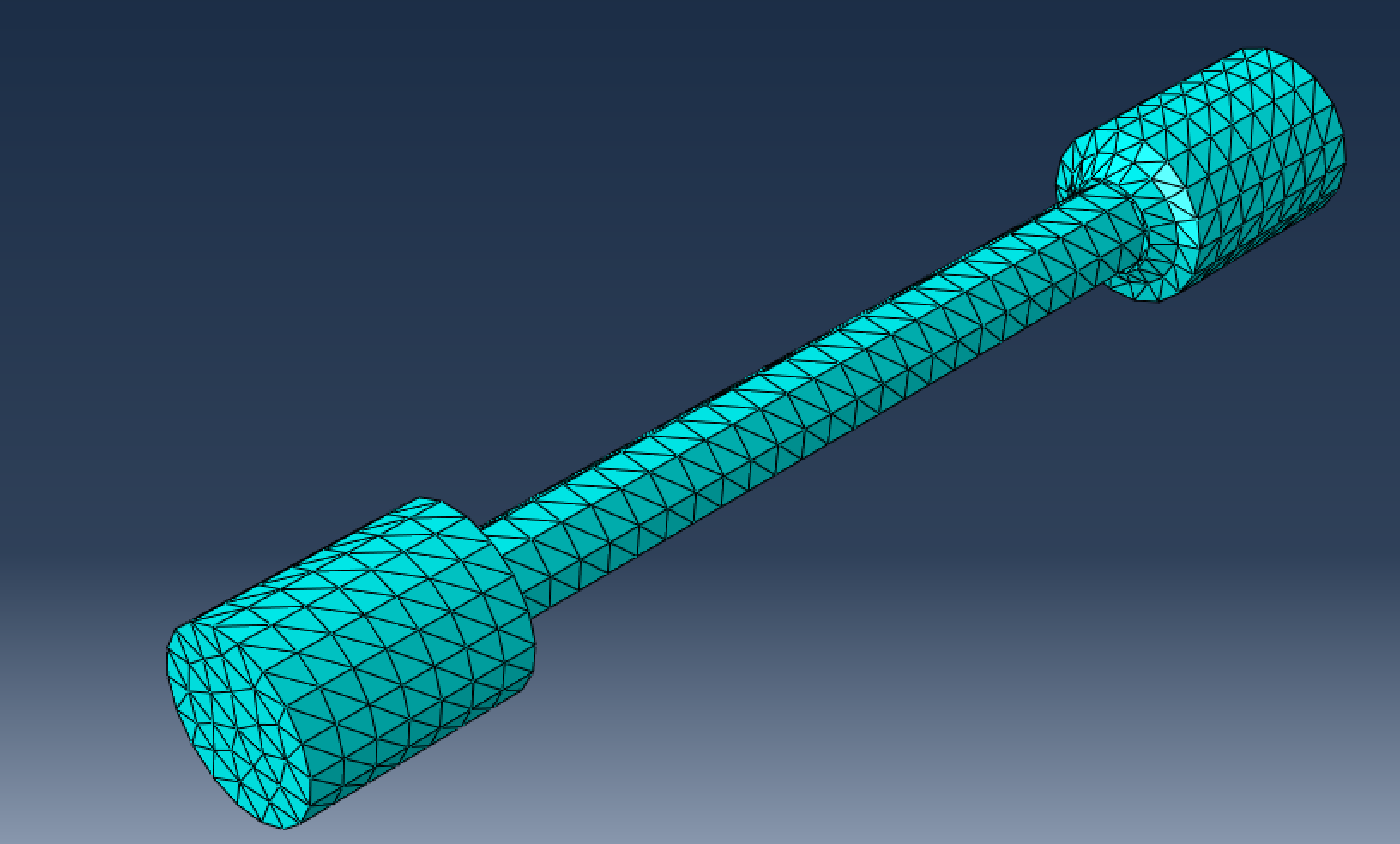
We requested 200 field output intervals in Abaqus, allowing us to inspect both global response curves and time-resolved necking and fracture progression. We reconstructed engineering stress–strain curves from displacement and reaction force at the loaded grip, and verified stress and strain over the 70 mm gauge section to obtain true stress–strain curves for comparison. This ensured consistent geometric baselines across numerical and experimental data.
Global curves indicate overall force and elongation, but cannot alone confirm whether the fracture process is physically sound. Therefore, we evaluated four categories of output simultaneously: stress S and equivalent plastic strain PEEQ to identify stress concentrations and plastic localization; damage variable SDEG and element status STATUS to track damage accumulation and element deletion; displacement and reaction force for curve reconstruction; and kinetic energy ALLKE versus internal energy ALLIE for quasi-static inertia verification.
This holistic approach dictated our evaluation criteria. While summarizes overall curve agreement, we did not rely on a single metric, evaluating necking profile, stress concentration locations, and element deletion timing in concert.
Mesh Sensitivity Study
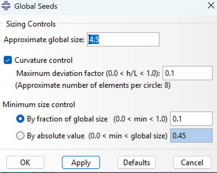
Due to local hardware constraints and node limits in the Abaqus Learning Edition, mesh refinement was bounded. Mesh M2 used an approximate global seed size of 4.5 with curvature control enabled; three additional mesh variants were used to observe how discretization scale influences stress–strain curves and localized fracture zones.
We compared the baseline mesh, M1, M2, and M3 against the same experimental curve, evaluating curve fit and fracture zone behavior.
| Mesh | Elements | Key Characteristics | |
|---|---|---|---|
| Baseline mesh | 3,846 | 0.9308 | Continued hardening post-peak |
| M1 | 830 | 0.9653 | Strain localized to very few elements |
| M2 | 1,975 | 0.9663 | Captures necking and post-peak softening |
| M3 | 2,928 | 0.9497 | Excessive strain localization |
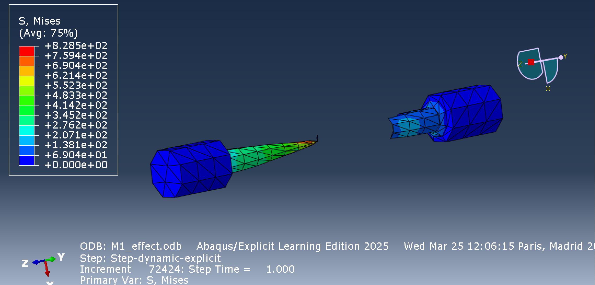
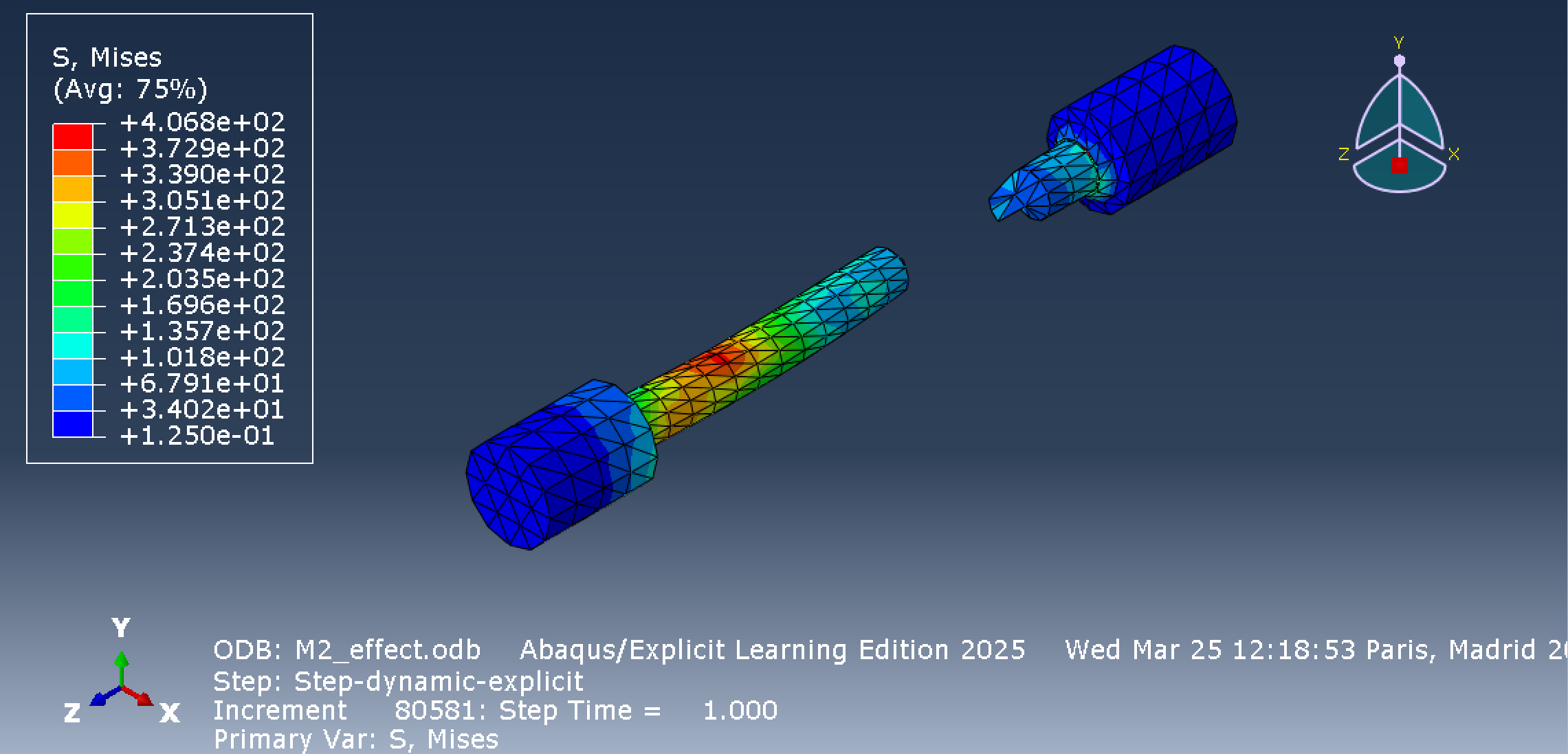
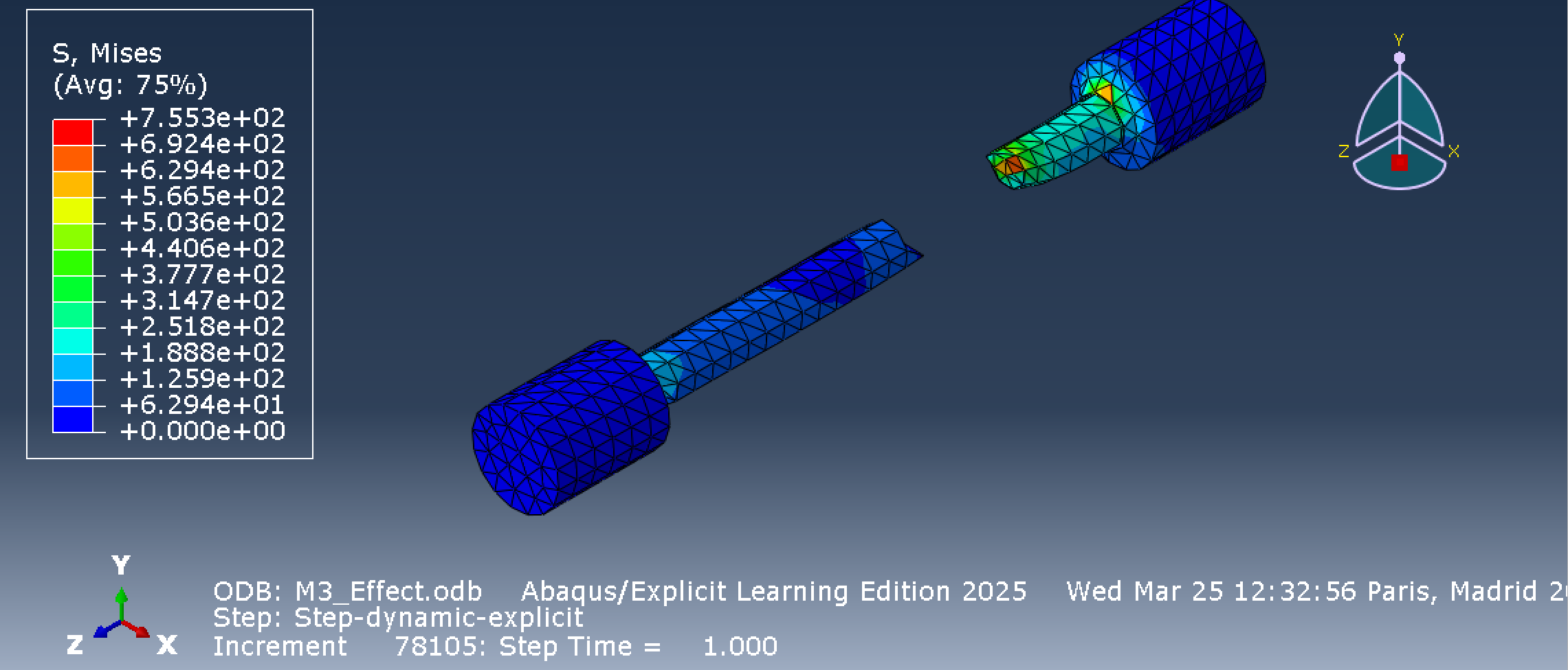
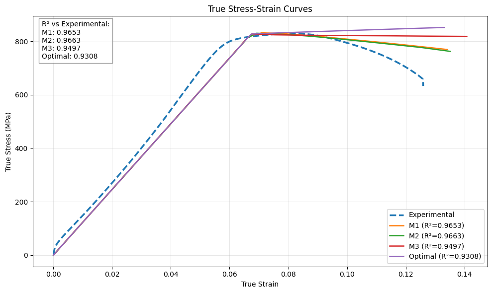
Mesh M1 contained only 830 elements, concentrating plastic strain into a very small number of cells. When element count was increased to 1,975 in M2, the simulation captured the experimentally observed necking and post-peak drop, achieving . Refining further to 2,928 elements in M3 caused damage to over-localize, dropping to 0.9497. Although the baseline mesh had 3,846 elements, it continued hardening post-peak, diverging from experimental softening.
These observations demonstrate that with damage models and element deletion, element size strongly influences the timing and spatial distribution of strain localization and erosion. Weighing global curve agreement, necking profile, stress distribution, and deletion behavior, we selected M2. This represents a pragmatic configuration choice under current tool constraints, rather than a claim of formal mesh convergence.
With the mesh established, the next question was: which solver configuration could reliably advance the simulation through material softening to final separation?
Comparing Solver Formulations
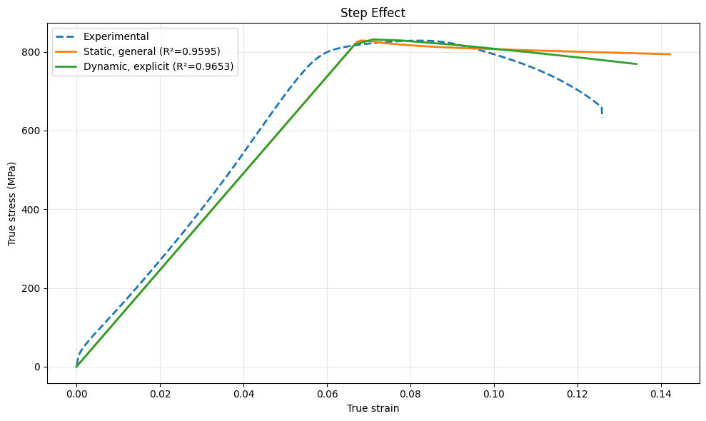
Our project archive preserves models solved with both Static General and Dynamic Explicit procedures. When Static General entered the necking and damage regimes, material softening introduced negative tangent stiffness, causing convergence difficulties and yielding a curve fit of . Dynamic Explicit avoids implicit Newton-Raphson iterations, smoothly tracking through damage evolution and element deletion to achieve an in reference runs.
Because displacement and damage parameter settings differed slightly between these archived models, they should not be viewed as an isolated single-variable solver benchmark. The 0.9653 value represents this specific Explicit reference run and is distinct from the 0.9663 achieved by the final M2 configuration. We selected Explicit primarily for its ability to calculate through post-peak softening and element deletion without numerical divergence, rather than relying solely on to claim universal superiority over Static solvers.
However, switching to Explicit introduces a new challenge: physical tensile testing is quasi-static, whereas explicit dynamics can inadvertently introduce spurious inertial effects. Next, we needed to verify that inertia did not dominate the response.
Quasi-Static Energy Checks for Explicit Dynamics
We monitored kinetic energy ALLKE and internal energy ALLIE to assess inertial effects. A Smooth Step amplitude profile ramps velocity and acceleration smoothly at the start and end of loading. In contrast, a linear Ramp induces sudden initial acceleration with subsequent oscillations, while an instantaneous Step behaves like an impact load.
In the Smooth Step simulation, the ratio ALLKE/ALLIE remained below 5% prior to fracture, with kinetic energy spikes appearing primarily during sudden element deletion at rupture. This satisfied our criteria for quasi-static validity, though it does not replace exhaustive dynamic verification.
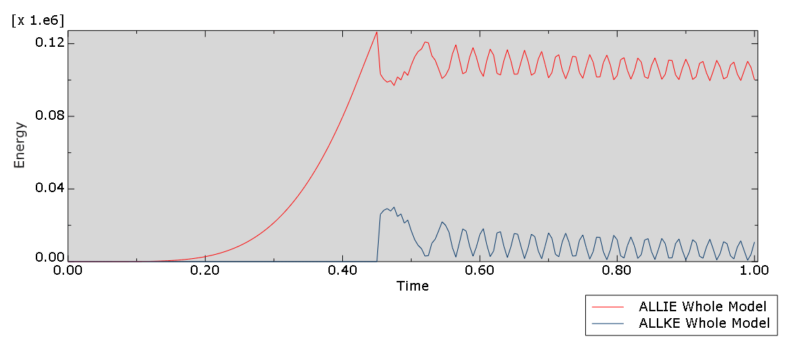
Loading amplitude directly influenced this energy balance across the three tested configurations:
| Loading Amplitude | Observed Behavior |
|---|---|
| Smooth Step | ALLKE/ALLIE remained below 5% prior to fracture |
| Linear Ramp | Initial inertial shock and transient oscillations |
| Instantaneous Step | Severe dynamic impact response |
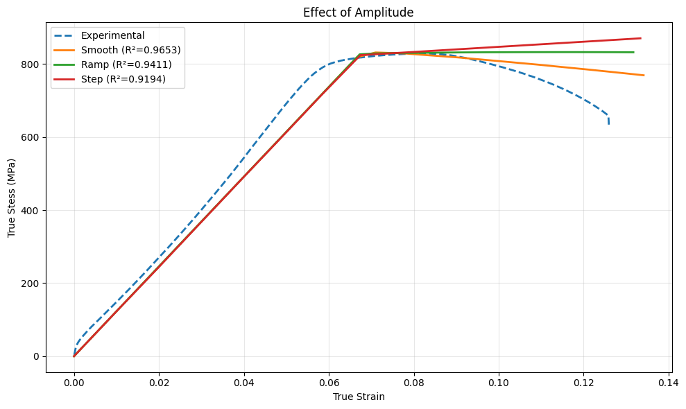
Consequently, Smooth Step was adopted for the final model configuration. With geometry, constitutive properties, mesh, solver, and amplitude each systematically justified, we evaluated the final numerical curve against experimental data.
Evaluating Final Model Fidelity
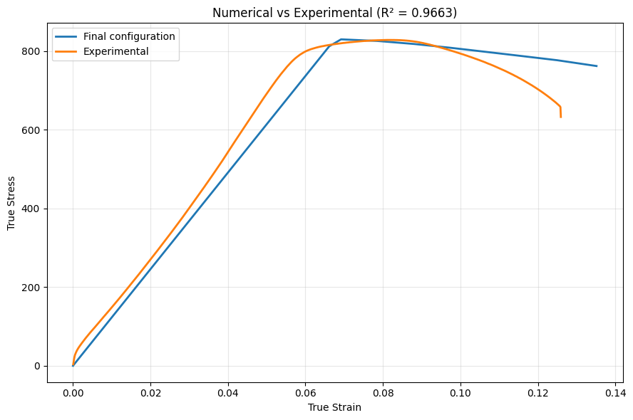
The final model configuration combined Mesh M2 + Dynamic Explicit + Smooth Step loading, yielding an overall curve correlation of . Prior to peak stress, the numerical curve accurately followed experimental plastic hardening trends; the simulated peak true stress reached approximately 820 MPa compared to the experimental 828.4 MPa—a difference of roughly 1%.
Beyond the peak, the specimen experienced necking, damage accumulation, and subsequent element deletion, with the numerical curve declining accordingly. A noticeable discrepancy remains: the tail of the numerical curve softens more gradually, remaining higher than experimental measurements. Thus, reflects strong global alignment rather than perfect pointwise agreement. Agreement is high around peak stress, while post-peak softening and the final rupture tail represent qualitative trend capture.
Summary
Reviewing this course project, we first corrected specimen geometry to derive valid material constitutive inputs from measured data; selected Mesh M2 based on curve fit, necking profile, stress distribution, and element deletion; retained the Dynamic Explicit procedure to handle post-peak softening and fracture; and employed a Smooth Step amplitude to suppress inertial shocks. Finally, we benchmarked the numerical curve against experimental data across hardening, peak stress, and post-peak softening regimes.
Several limitations apply to these findings: the dataset is derived from a single tensile test without statistical confidence intervals, and damage parameters were calibrated against the same test curve. The low apparent modulus reflects compliance from the machine frame and grips, and the Abaqus Learning Edition constrained allowable mesh refinement.
Nevertheless, this project provided clear insight into why the specimen fractured under these specific numerical configurations, as well as which regions of the simulated response are robust and which require engineering judgment. It proved to be a valuable end-to-end exercise in FEA digital twin modeling.